2.2: Lab 2 - Cross-sections and Three-point Problems
- Page ID
- 12506
\( \newcommand{\vecs}[1]{\overset { \scriptstyle \rightharpoonup} {\mathbf{#1}} } \)
\( \newcommand{\vecd}[1]{\overset{-\!-\!\rightharpoonup}{\vphantom{a}\smash {#1}}} \)
\( \newcommand{\id}{\mathrm{id}}\) \( \newcommand{\Span}{\mathrm{span}}\)
( \newcommand{\kernel}{\mathrm{null}\,}\) \( \newcommand{\range}{\mathrm{range}\,}\)
\( \newcommand{\RealPart}{\mathrm{Re}}\) \( \newcommand{\ImaginaryPart}{\mathrm{Im}}\)
\( \newcommand{\Argument}{\mathrm{Arg}}\) \( \newcommand{\norm}[1]{\| #1 \|}\)
\( \newcommand{\inner}[2]{\langle #1, #2 \rangle}\)
\( \newcommand{\Span}{\mathrm{span}}\)
\( \newcommand{\id}{\mathrm{id}}\)
\( \newcommand{\Span}{\mathrm{span}}\)
\( \newcommand{\kernel}{\mathrm{null}\,}\)
\( \newcommand{\range}{\mathrm{range}\,}\)
\( \newcommand{\RealPart}{\mathrm{Re}}\)
\( \newcommand{\ImaginaryPart}{\mathrm{Im}}\)
\( \newcommand{\Argument}{\mathrm{Arg}}\)
\( \newcommand{\norm}[1]{\| #1 \|}\)
\( \newcommand{\inner}[2]{\langle #1, #2 \rangle}\)
\( \newcommand{\Span}{\mathrm{span}}\) \( \newcommand{\AA}{\unicode[.8,0]{x212B}}\)
\( \newcommand{\vectorA}[1]{\vec{#1}} % arrow\)
\( \newcommand{\vectorAt}[1]{\vec{\text{#1}}} % arrow\)
\( \newcommand{\vectorB}[1]{\overset { \scriptstyle \rightharpoonup} {\mathbf{#1}} } \)
\( \newcommand{\vectorC}[1]{\textbf{#1}} \)
\( \newcommand{\vectorD}[1]{\overrightarrow{#1}} \)
\( \newcommand{\vectorDt}[1]{\overrightarrow{\text{#1}}} \)
\( \newcommand{\vectE}[1]{\overset{-\!-\!\rightharpoonup}{\vphantom{a}\smash{\mathbf {#1}}}} \)
\( \newcommand{\vecs}[1]{\overset { \scriptstyle \rightharpoonup} {\mathbf{#1}} } \)
\( \newcommand{\vecd}[1]{\overset{-\!-\!\rightharpoonup}{\vphantom{a}\smash {#1}}} \)
\(\newcommand{\avec}{\mathbf a}\) \(\newcommand{\bvec}{\mathbf b}\) \(\newcommand{\cvec}{\mathbf c}\) \(\newcommand{\dvec}{\mathbf d}\) \(\newcommand{\dtil}{\widetilde{\mathbf d}}\) \(\newcommand{\evec}{\mathbf e}\) \(\newcommand{\fvec}{\mathbf f}\) \(\newcommand{\nvec}{\mathbf n}\) \(\newcommand{\pvec}{\mathbf p}\) \(\newcommand{\qvec}{\mathbf q}\) \(\newcommand{\svec}{\mathbf s}\) \(\newcommand{\tvec}{\mathbf t}\) \(\newcommand{\uvec}{\mathbf u}\) \(\newcommand{\vvec}{\mathbf v}\) \(\newcommand{\wvec}{\mathbf w}\) \(\newcommand{\xvec}{\mathbf x}\) \(\newcommand{\yvec}{\mathbf y}\) \(\newcommand{\zvec}{\mathbf z}\) \(\newcommand{\rvec}{\mathbf r}\) \(\newcommand{\mvec}{\mathbf m}\) \(\newcommand{\zerovec}{\mathbf 0}\) \(\newcommand{\onevec}{\mathbf 1}\) \(\newcommand{\real}{\mathbb R}\) \(\newcommand{\twovec}[2]{\left[\begin{array}{r}#1 \\ #2 \end{array}\right]}\) \(\newcommand{\ctwovec}[2]{\left[\begin{array}{c}#1 \\ #2 \end{array}\right]}\) \(\newcommand{\threevec}[3]{\left[\begin{array}{r}#1 \\ #2 \\ #3 \end{array}\right]}\) \(\newcommand{\cthreevec}[3]{\left[\begin{array}{c}#1 \\ #2 \\ #3 \end{array}\right]}\) \(\newcommand{\fourvec}[4]{\left[\begin{array}{r}#1 \\ #2 \\ #3 \\ #4 \end{array}\right]}\) \(\newcommand{\cfourvec}[4]{\left[\begin{array}{c}#1 \\ #2 \\ #3 \\ #4 \end{array}\right]}\) \(\newcommand{\fivevec}[5]{\left[\begin{array}{r}#1 \\ #2 \\ #3 \\ #4 \\ #5 \\ \end{array}\right]}\) \(\newcommand{\cfivevec}[5]{\left[\begin{array}{c}#1 \\ #2 \\ #3 \\ #4 \\ #5 \\ \end{array}\right]}\) \(\newcommand{\mattwo}[4]{\left[\begin{array}{rr}#1 \amp #2 \\ #3 \amp #4 \\ \end{array}\right]}\) \(\newcommand{\laspan}[1]{\text{Span}\{#1\}}\) \(\newcommand{\bcal}{\cal B}\) \(\newcommand{\ccal}{\cal C}\) \(\newcommand{\scal}{\cal S}\) \(\newcommand{\wcal}{\cal W}\) \(\newcommand{\ecal}{\cal E}\) \(\newcommand{\coords}[2]{\left\{#1\right\}_{#2}}\) \(\newcommand{\gray}[1]{\color{gray}{#1}}\) \(\newcommand{\lgray}[1]{\color{lightgray}{#1}}\) \(\newcommand{\rank}{\operatorname{rank}}\) \(\newcommand{\row}{\text{Row}}\) \(\newcommand{\col}{\text{Col}}\) \(\renewcommand{\row}{\text{Row}}\) \(\newcommand{\nul}{\text{Nul}}\) \(\newcommand{\var}{\text{Var}}\) \(\newcommand{\corr}{\text{corr}}\) \(\newcommand{\len}[1]{\left|#1\right|}\) \(\newcommand{\bbar}{\overline{\bvec}}\) \(\newcommand{\bhat}{\widehat{\bvec}}\) \(\newcommand{\bperp}{\bvec^\perp}\) \(\newcommand{\xhat}{\widehat{\xvec}}\) \(\newcommand{\vhat}{\widehat{\vvec}}\) \(\newcommand{\uhat}{\widehat{\uvec}}\) \(\newcommand{\what}{\widehat{\wvec}}\) \(\newcommand{\Sighat}{\widehat{\Sigma}}\) \(\newcommand{\lt}{<}\) \(\newcommand{\gt}{>}\) \(\newcommand{\amp}{&}\) \(\definecolor{fillinmathshade}{gray}{0.9}\)Topographic profiles and cross-sections
Topographic profiles show the shape of the Earth’s surface in a view that simulates a vertical slice through the landscape. Topographic profiles may be constructed by noting where topographic contours cross the line of the profile.
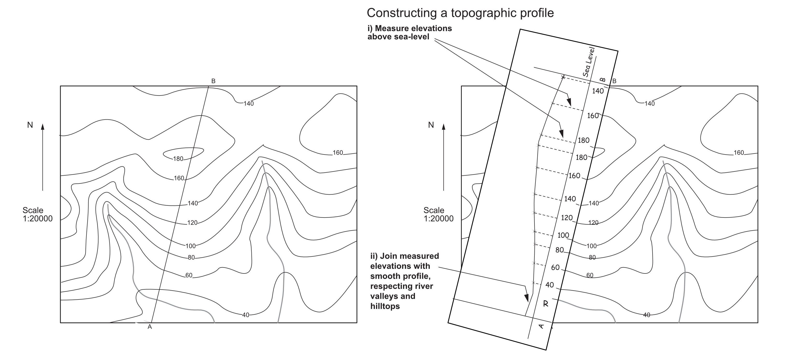
You may remember the technique for drawing a topographic profile from your introductory geology course (Fig. 1). On a profile or a cross-section, the ratio of the vertical scale to the horizontal scale, expressed as a fraction, is the vertical exaggeration. If the vertical and horizontal scales are equal the section is said to have a natural scale. Unless there is a good reason to use vertical exaggeration, it is generally best in structural geology to draw sections at natural scale.
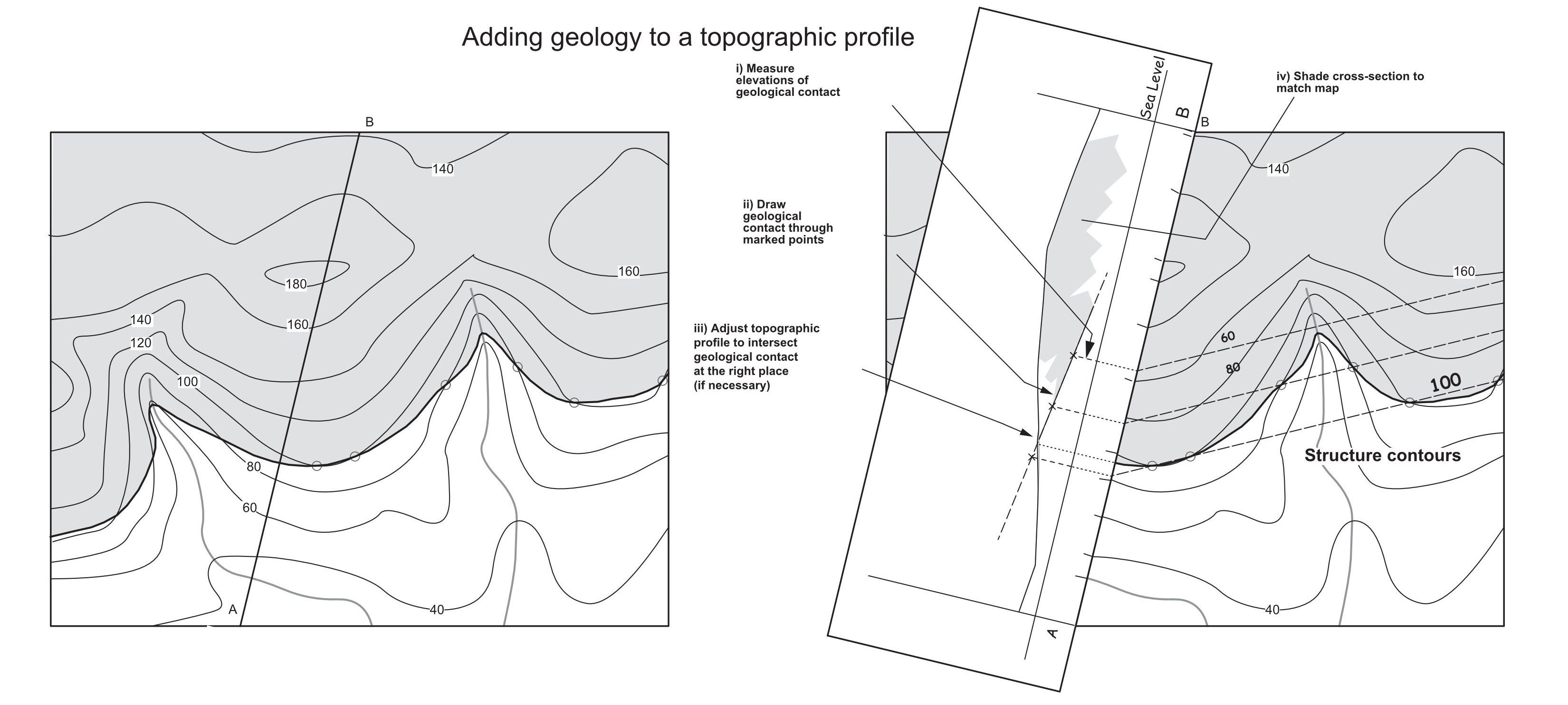
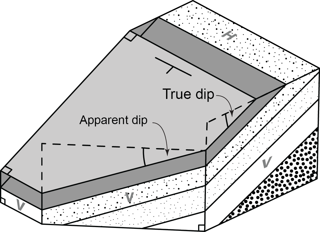
A vertical cross-section showing the trace of a geologic surface may be constructed in exactly the same way by noting where structure contours cross the line of section. Where a natural scale has been used and the line of section is perpendicular to the strike, the cross-section shows the true dip. On sections oblique to strike, the cross-section shows the apparent dip. It is possible to demonstrate that apparent dip is always less than true dip. Figure 3 shows apparent dip and true dip in different cross-sections.
In a cross-section through a succession containing an angular unconformity, there is no possible orientation of the cross-section that will show true dip for both the underlying and overlying parts of the succession, unless they both have the same strike. Cross-sections with vertical exaggeration show neither true nor apparent dip.
Three-point problems
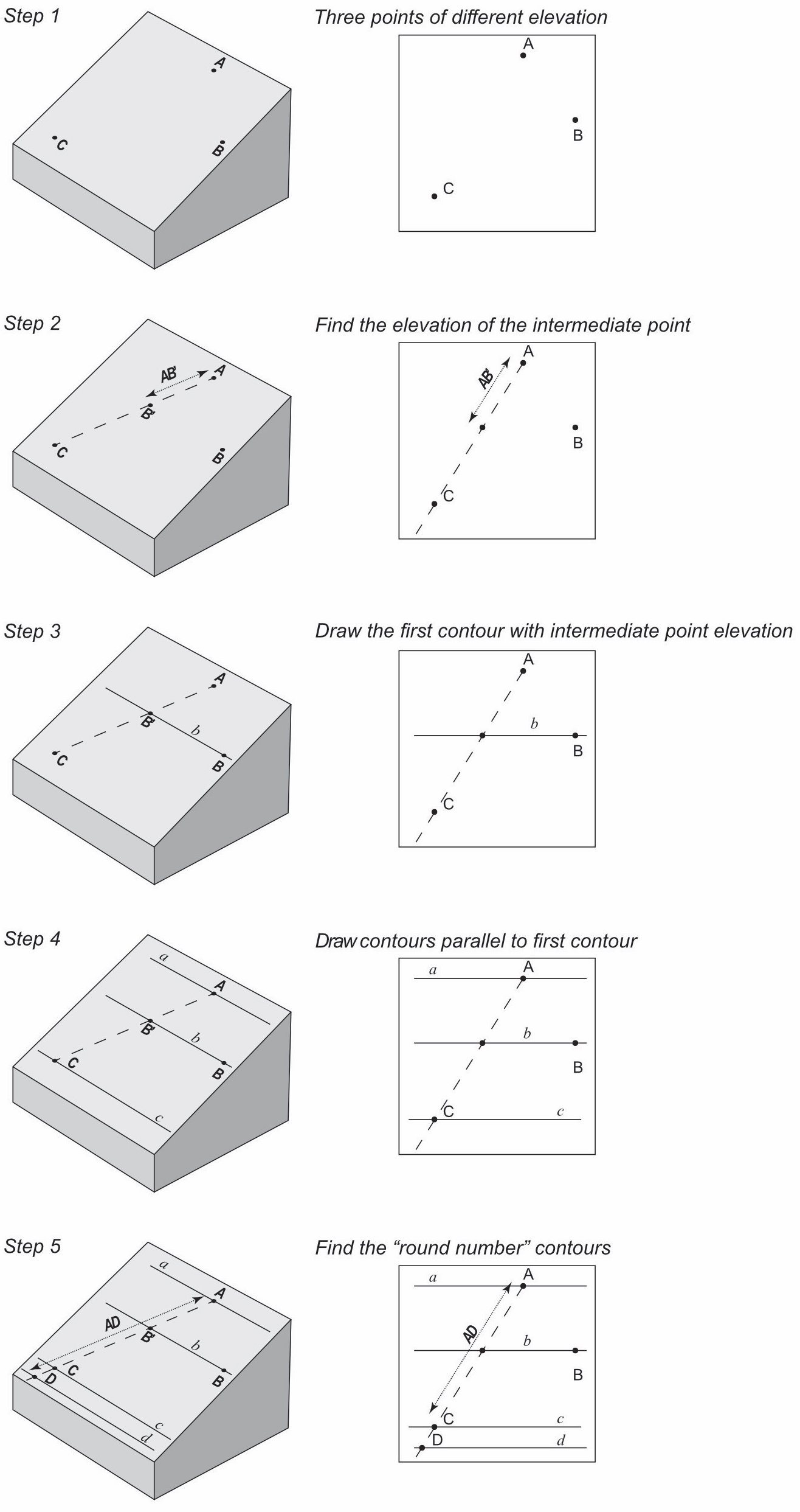
Structure contours may be drawn for a planar surface if we know its elevation at three points. This is known as a ‘three point problem’.
You need three points of known location and elevation all plotted on a map (Fig. 4). One of these points must be the highest – it’s labelled A in the diagram. One is the lowest, labelled C. The intermediate point is B. The elevations of the three points are represented in the following by lowercase letters a, b, c, from highest to lowest.
The first step in solving the problem is to connect the high and low points on the map with a line AC. Somewhere along this line there will be a point (call it B’) with the same elevation as B. The distance of B’ along line AC is proportional to the height differences.
In other words: (Length AB’) / (Length AC) = (a-b) / (a-c)
so (Length AB’) = (Length AC) × (a-b) / (a-c)
Use this relationship to locate B’, and join B and B’ with a line. This is your first structure contour.
Since we are assuming this is a planar surface, we can also draw two more contours at elevations a and c
It’s unlikely that a, b or c is a ’round number’ like 200 or 5000, comparable with the topographic contours on the map. There are several ways to find a contour with a round number value (call it d). Probably the easiest is to repeat the calculation above, to locate a point with elevation d that lies on line AC:
(Length AD) = (Length AC) × (a-d) / (a-c)
Note that in the example, point D lies beyond the end of line AC, but this is not necessarily the case; the same method can be used to find contours that pass between A and C.
Assignment
1.* Examine the geological map of the Grand Canyon. Even without structure contours, we can make some inferences about the orientations of different geological units.
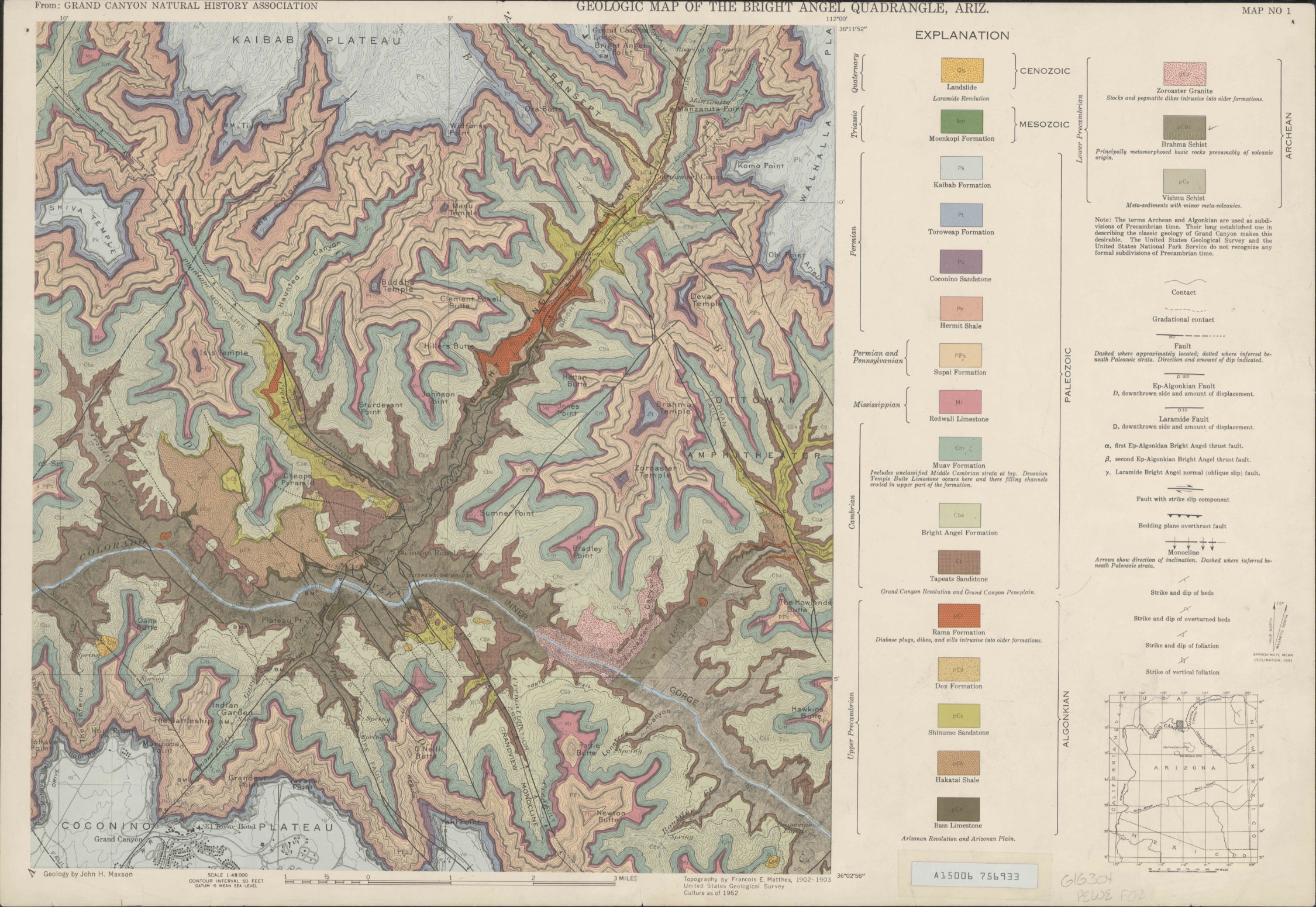
Link to larger version of map
Look at the topographic contours and notice that their spacing varies dramatically. In some places they are widely spaced, whereas in others they are so close together that they merge together. The steepest slopes are typically found on particular geologic units of erosion-resistant rocks, known as ‘cliff-forming’ units.
a) Using the legend, identify and name one cliff-forming Paleozoic unit that outcrops in consistently steep topographic slopes.
In addition to information about erosion-resistance, the map pattern carries information about the dip of units. Based on the map pattern, what can you say about the dip of the following units? (In each case, your answer should be something like ‘approximately horizontal’, ‘approximately vertical’, ‘dipping gently’, etc.)
b) The Archean units
c) The Algonquian units
d) The Paleozoic units
e) The Bright Angel Fault
In addition, the map gives you information about geologic time, both by the principle of superposition (younger rocks on top of older) and by the principle of cross-cutting relationships (older structures are cut by younger). An angular unconformity is a type of cross-cutting relationship where a younger unit lies on the eroded surfaces of many different older units.
f) Look for unconformities that are visible in the map pattern and identify two. In each case, specify which unit lies immediately above the unconformity surface. (This is the best way to specify the location of an unconformity in a stratigraphic succession because typically a single upper unit lies on a variety of lower units). For each unconformity, say which units of rock are overstepped, and also mention any evidence for onlap at the unconformity surface.
g) There is at least one more unconformity on the map but it is a disconformity, so there is no cross-cutting relationship. Using the legend and your knowledge of the geologic timescale, identify its location in the stratigraphy.
2. Map 1 shows the trace of an unconformable contact between slate and an overlying conglomerate. Conformably overlying the conglomerate is sandstone and limestone.
Lab 2, Map 1: Stratified units overlying slate with veins
a. Draw structure contours on the unconformity surface.
b. Determine its orientation (strike and dip).
c. Draw structure contours on the remaining contacts. You may notice that some structure contours are shared between multiple surfaces. Draw the structure contours in pencil and label each surface with a different colour.
d. Draw two vertical topographic profiles with bearings of 099o and 000o through the point P. You may remember the technique for drawing a topographic profile from your introductory geology course. The scale of the map is 1:7500. Your topographic profiles should be drawn at natural scale(no vertical exaggeration).
e. Now add the unconformity to the topographic profile to make a cross section. To do this, use the intersections of structure contours with the profile in exactly the same way you used the intersections of topographic contours in the previous question! (Do not try to use the calculated dip to place the plane on the cross section; if the cross-section is at an angle to the dip it will show an apparent dip, not a true dip. By far the easiest and most accurate way to place surfaces on the section is by using the structure contours. Also, the contour technique always works even if you have to construct a vertically exaggerated section.) If you do not have enough contours to constrain the surface on the cross-section, interpolate contours at intermediate elevations (325, 350, 375 m etc.).
f. Complete the sections by adding in the remaining surfaces and shade the units with appropriate patterns.
*g. Which of the slopes of the traces of the unconformity on the above cross-sections equals the true dip and which an apparent dip?
*h. A copy of Map 1 is provided in next week’s lab. Enter your answer from part b in the space provided above the map, as you will need to use these numbers.
3. Also on Map 1 is a dotted line representing the trace of a gold-bearing vein in slates exposed on the hillside at S. A planar gold-bearing vein was also intersected in borehole Q, 100 m below the topographic surface, and in borehole T, 300 m below the surface. Assuming all three observations are of the same gold vein, you have enough information to determine its orientation.
Use the 3-point method to draw structure contours on the vein.
a. Determine its strike and dip.
b. Draw the subcrop line of the vein by finding the intersection of the two sets of structure contours.
c. Determine the trend and plunge of this line.
d. Complete the outcrop pattern of the vein on the map.
e. Add the vein to both cross-sections.
f. * A prospector suggests drilling through the outlier at Y to look for the gold vein below the unconformity. Explain why this suggestion would be a bad idea.
g. * The prospector then suggests drilling through the inlier at X to look for the gold vein below the unconformity. Explain why this suggestion would also be a bad idea.
h. * Enter your answers from parts b and d in the spaces provided above the map in next week’s lab, as you will need to use these numbers.


