
14.4: Activity 14C - T-charts, Decay Curves, and Half-lives
- Page ID
- 14848

\( \newcommand{\vecs}[1]{\overset { \scriptstyle \rightharpoonup} {\mathbf{#1}} } \)
\( \newcommand{\vecd}[1]{\overset{-\!-\!\rightharpoonup}{\vphantom{a}\smash {#1}}} \)
\( \newcommand{\id}{\mathrm{id}}\) \( \newcommand{\Span}{\mathrm{span}}\)
( \newcommand{\kernel}{\mathrm{null}\,}\) \( \newcommand{\range}{\mathrm{range}\,}\)
\( \newcommand{\RealPart}{\mathrm{Re}}\) \( \newcommand{\ImaginaryPart}{\mathrm{Im}}\)
\( \newcommand{\Argument}{\mathrm{Arg}}\) \( \newcommand{\norm}[1]{\| #1 \|}\)
\( \newcommand{\inner}[2]{\langle #1, #2 \rangle}\)
\( \newcommand{\Span}{\mathrm{span}}\)
\( \newcommand{\id}{\mathrm{id}}\)
\( \newcommand{\Span}{\mathrm{span}}\)
\( \newcommand{\kernel}{\mathrm{null}\,}\)
\( \newcommand{\range}{\mathrm{range}\,}\)
\( \newcommand{\RealPart}{\mathrm{Re}}\)
\( \newcommand{\ImaginaryPart}{\mathrm{Im}}\)
\( \newcommand{\Argument}{\mathrm{Arg}}\)
\( \newcommand{\norm}[1]{\| #1 \|}\)
\( \newcommand{\inner}[2]{\langle #1, #2 \rangle}\)
\( \newcommand{\Span}{\mathrm{span}}\) \( \newcommand{\AA}{\unicode[.8,0]{x212B}}\)
\( \newcommand{\vectorA}[1]{\vec{#1}} % arrow\)
\( \newcommand{\vectorAt}[1]{\vec{\text{#1}}} % arrow\)
\( \newcommand{\vectorB}[1]{\overset { \scriptstyle \rightharpoonup} {\mathbf{#1}} } \)
\( \newcommand{\vectorC}[1]{\textbf{#1}} \)
\( \newcommand{\vectorD}[1]{\overrightarrow{#1}} \)
\( \newcommand{\vectorDt}[1]{\overrightarrow{\text{#1}}} \)
\( \newcommand{\vectE}[1]{\overset{-\!-\!\rightharpoonup}{\vphantom{a}\smash{\mathbf {#1}}}} \)
\( \newcommand{\vecs}[1]{\overset { \scriptstyle \rightharpoonup} {\mathbf{#1}} } \)
\( \newcommand{\vecd}[1]{\overset{-\!-\!\rightharpoonup}{\vphantom{a}\smash {#1}}} \)
\(\newcommand{\avec}{\mathbf a}\) \(\newcommand{\bvec}{\mathbf b}\) \(\newcommand{\cvec}{\mathbf c}\) \(\newcommand{\dvec}{\mathbf d}\) \(\newcommand{\dtil}{\widetilde{\mathbf d}}\) \(\newcommand{\evec}{\mathbf e}\) \(\newcommand{\fvec}{\mathbf f}\) \(\newcommand{\nvec}{\mathbf n}\) \(\newcommand{\pvec}{\mathbf p}\) \(\newcommand{\qvec}{\mathbf q}\) \(\newcommand{\svec}{\mathbf s}\) \(\newcommand{\tvec}{\mathbf t}\) \(\newcommand{\uvec}{\mathbf u}\) \(\newcommand{\vvec}{\mathbf v}\) \(\newcommand{\wvec}{\mathbf w}\) \(\newcommand{\xvec}{\mathbf x}\) \(\newcommand{\yvec}{\mathbf y}\) \(\newcommand{\zvec}{\mathbf z}\) \(\newcommand{\rvec}{\mathbf r}\) \(\newcommand{\mvec}{\mathbf m}\) \(\newcommand{\zerovec}{\mathbf 0}\) \(\newcommand{\onevec}{\mathbf 1}\) \(\newcommand{\real}{\mathbb R}\) \(\newcommand{\twovec}[2]{\left[\begin{array}{r}#1 \\ #2 \end{array}\right]}\) \(\newcommand{\ctwovec}[2]{\left[\begin{array}{c}#1 \\ #2 \end{array}\right]}\) \(\newcommand{\threevec}[3]{\left[\begin{array}{r}#1 \\ #2 \\ #3 \end{array}\right]}\) \(\newcommand{\cthreevec}[3]{\left[\begin{array}{c}#1 \\ #2 \\ #3 \end{array}\right]}\) \(\newcommand{\fourvec}[4]{\left[\begin{array}{r}#1 \\ #2 \\ #3 \\ #4 \end{array}\right]}\) \(\newcommand{\cfourvec}[4]{\left[\begin{array}{c}#1 \\ #2 \\ #3 \\ #4 \end{array}\right]}\) \(\newcommand{\fivevec}[5]{\left[\begin{array}{r}#1 \\ #2 \\ #3 \\ #4 \\ #5 \\ \end{array}\right]}\) \(\newcommand{\cfivevec}[5]{\left[\begin{array}{c}#1 \\ #2 \\ #3 \\ #4 \\ #5 \\ \end{array}\right]}\) \(\newcommand{\mattwo}[4]{\left[\begin{array}{rr}#1 \amp #2 \\ #3 \amp #4 \\ \end{array}\right]}\) \(\newcommand{\laspan}[1]{\text{Span}\{#1\}}\) \(\newcommand{\bcal}{\cal B}\) \(\newcommand{\ccal}{\cal C}\) \(\newcommand{\scal}{\cal S}\) \(\newcommand{\wcal}{\cal W}\) \(\newcommand{\ecal}{\cal E}\) \(\newcommand{\coords}[2]{\left\{#1\right\}_{#2}}\) \(\newcommand{\gray}[1]{\color{gray}{#1}}\) \(\newcommand{\lgray}[1]{\color{lightgray}{#1}}\) \(\newcommand{\rank}{\operatorname{rank}}\) \(\newcommand{\row}{\text{Row}}\) \(\newcommand{\col}{\text{Col}}\) \(\renewcommand{\row}{\text{Row}}\) \(\newcommand{\nul}{\text{Nul}}\) \(\newcommand{\var}{\text{Var}}\) \(\newcommand{\corr}{\text{corr}}\) \(\newcommand{\len}[1]{\left|#1\right|}\) \(\newcommand{\bbar}{\overline{\bvec}}\) \(\newcommand{\bhat}{\widehat{\bvec}}\) \(\newcommand{\bperp}{\bvec^\perp}\) \(\newcommand{\xhat}{\widehat{\xvec}}\) \(\newcommand{\vhat}{\widehat{\vvec}}\) \(\newcommand{\uhat}{\widehat{\uvec}}\) \(\newcommand{\what}{\widehat{\wvec}}\) \(\newcommand{\Sighat}{\widehat{\Sigma}}\) \(\newcommand{\lt}{<}\) \(\newcommand{\gt}{>}\) \(\newcommand{\amp}{&}\) \(\definecolor{fillinmathshade}{gray}{0.9}\)Helpful tips to calculate a half-life:
- Draw or insert a T-chart.
- In the T-chart, label the left side with time units (number of half-lives, years, ka, Ma, Ga, etc.)
- Label right side with mass units (percentage, atoms, gram, kilograms, etc.)
- Begin by ALWAYS writing zero in the first spot of the time column.
- In the mass column, begin with the given mass if provided. Recall that this is 100% of the original parent isotope.
- If the mass is the starting mass, keep dividing the number in the mass column by 2 for each half-life in the left column.
- If you are given a final mass, record this at the very bottom of the mass column.
- If the mass given is the final mass, multiply that mass by 2 until the initial time (Time 0) is reached.
- The final mass amount at the bottom of the mass column equals how much mass is left after radioactive decay has occurred.
- In the time column, add one half-life at a time until you reach the total time given in problem. The number of half-lives elapsed is equal to the number of times you added a half-life in the time column.
1. Calculate the amount of parent isotope remaining for all the given half-lives in this T-chart.
| Number of Half-lives | Amount of Parent Isotope Remaining (%) |
|---|---|
| 0 | 100 |
| 1 | |
| 2 | |
| 3 | |
| 4 | |
| 5 | |
| 6 | |
| 7 | |
| 8 |
2. Plot your findings from the T-chart on the graph below.
3. Draw the decay curve by connecting your plotted data points.
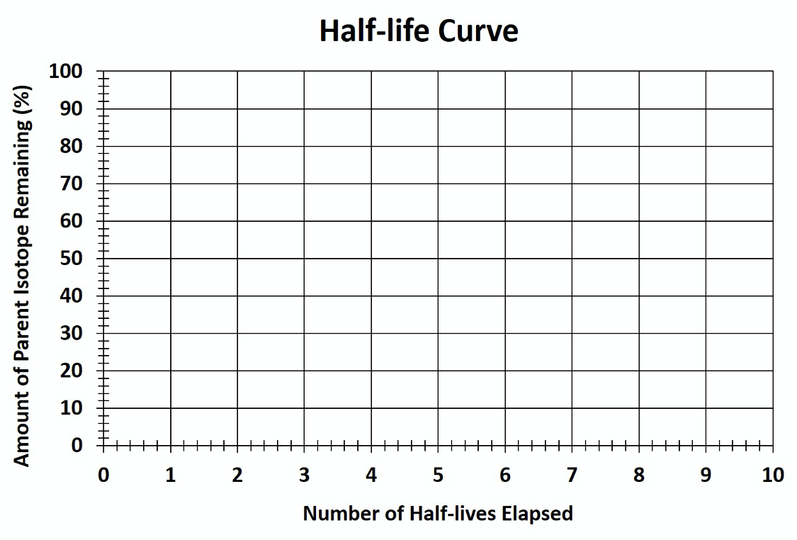
Using the above graph (Figure 14.25), answer the following questions.
4. How much of the parent isotope would be remaining after 7 half-lives have passed?
a. 6.25%
b. 1.56%
c. 0.78%
d. 0.39%
5. If a radiometric element has a half-life of 425 years, how old would a rock be that only had 3.125% of the parent isotope remaining?
a. 2125 years
b. 1700 years
c. 2550 years
d. 3400 years
6. Approximately how much of the parent isotope would be remaining after 3.5 half-lives?
a. 16%
b. 12%
c. 4%
d. 8%
7. Based on your graph above, approximately how many half-lives have passed when only 35% of the parent isotope is remaining?
a. 0.75
b. 1.5
c. 2.1
d. 2.5
Attributions
- Table 14.4: “T-Chart” (CC-BY 4.0; Chloe Branciforte, own work)
- Figure 14.25: “Half-life Curve Graph” (CC-BY 4.0; Chloe Branciforte, own work)