9.2.1: Characteristics of a Boomtown
- Page ID
- 15684
\( \newcommand{\vecs}[1]{\overset { \scriptstyle \rightharpoonup} {\mathbf{#1}} } \)
\( \newcommand{\vecd}[1]{\overset{-\!-\!\rightharpoonup}{\vphantom{a}\smash {#1}}} \)
\( \newcommand{\id}{\mathrm{id}}\) \( \newcommand{\Span}{\mathrm{span}}\)
( \newcommand{\kernel}{\mathrm{null}\,}\) \( \newcommand{\range}{\mathrm{range}\,}\)
\( \newcommand{\RealPart}{\mathrm{Re}}\) \( \newcommand{\ImaginaryPart}{\mathrm{Im}}\)
\( \newcommand{\Argument}{\mathrm{Arg}}\) \( \newcommand{\norm}[1]{\| #1 \|}\)
\( \newcommand{\inner}[2]{\langle #1, #2 \rangle}\)
\( \newcommand{\Span}{\mathrm{span}}\)
\( \newcommand{\id}{\mathrm{id}}\)
\( \newcommand{\Span}{\mathrm{span}}\)
\( \newcommand{\kernel}{\mathrm{null}\,}\)
\( \newcommand{\range}{\mathrm{range}\,}\)
\( \newcommand{\RealPart}{\mathrm{Re}}\)
\( \newcommand{\ImaginaryPart}{\mathrm{Im}}\)
\( \newcommand{\Argument}{\mathrm{Arg}}\)
\( \newcommand{\norm}[1]{\| #1 \|}\)
\( \newcommand{\inner}[2]{\langle #1, #2 \rangle}\)
\( \newcommand{\Span}{\mathrm{span}}\) \( \newcommand{\AA}{\unicode[.8,0]{x212B}}\)
\( \newcommand{\vectorA}[1]{\vec{#1}} % arrow\)
\( \newcommand{\vectorAt}[1]{\vec{\text{#1}}} % arrow\)
\( \newcommand{\vectorB}[1]{\overset { \scriptstyle \rightharpoonup} {\mathbf{#1}} } \)
\( \newcommand{\vectorC}[1]{\textbf{#1}} \)
\( \newcommand{\vectorD}[1]{\overrightarrow{#1}} \)
\( \newcommand{\vectorDt}[1]{\overrightarrow{\text{#1}}} \)
\( \newcommand{\vectE}[1]{\overset{-\!-\!\rightharpoonup}{\vphantom{a}\smash{\mathbf {#1}}}} \)
\( \newcommand{\vecs}[1]{\overset { \scriptstyle \rightharpoonup} {\mathbf{#1}} } \)
\( \newcommand{\vecd}[1]{\overset{-\!-\!\rightharpoonup}{\vphantom{a}\smash {#1}}} \)
\(\newcommand{\avec}{\mathbf a}\) \(\newcommand{\bvec}{\mathbf b}\) \(\newcommand{\cvec}{\mathbf c}\) \(\newcommand{\dvec}{\mathbf d}\) \(\newcommand{\dtil}{\widetilde{\mathbf d}}\) \(\newcommand{\evec}{\mathbf e}\) \(\newcommand{\fvec}{\mathbf f}\) \(\newcommand{\nvec}{\mathbf n}\) \(\newcommand{\pvec}{\mathbf p}\) \(\newcommand{\qvec}{\mathbf q}\) \(\newcommand{\svec}{\mathbf s}\) \(\newcommand{\tvec}{\mathbf t}\) \(\newcommand{\uvec}{\mathbf u}\) \(\newcommand{\vvec}{\mathbf v}\) \(\newcommand{\wvec}{\mathbf w}\) \(\newcommand{\xvec}{\mathbf x}\) \(\newcommand{\yvec}{\mathbf y}\) \(\newcommand{\zvec}{\mathbf z}\) \(\newcommand{\rvec}{\mathbf r}\) \(\newcommand{\mvec}{\mathbf m}\) \(\newcommand{\zerovec}{\mathbf 0}\) \(\newcommand{\onevec}{\mathbf 1}\) \(\newcommand{\real}{\mathbb R}\) \(\newcommand{\twovec}[2]{\left[\begin{array}{r}#1 \\ #2 \end{array}\right]}\) \(\newcommand{\ctwovec}[2]{\left[\begin{array}{c}#1 \\ #2 \end{array}\right]}\) \(\newcommand{\threevec}[3]{\left[\begin{array}{r}#1 \\ #2 \\ #3 \end{array}\right]}\) \(\newcommand{\cthreevec}[3]{\left[\begin{array}{c}#1 \\ #2 \\ #3 \end{array}\right]}\) \(\newcommand{\fourvec}[4]{\left[\begin{array}{r}#1 \\ #2 \\ #3 \\ #4 \end{array}\right]}\) \(\newcommand{\cfourvec}[4]{\left[\begin{array}{c}#1 \\ #2 \\ #3 \\ #4 \end{array}\right]}\) \(\newcommand{\fivevec}[5]{\left[\begin{array}{r}#1 \\ #2 \\ #3 \\ #4 \\ #5 \\ \end{array}\right]}\) \(\newcommand{\cfivevec}[5]{\left[\begin{array}{c}#1 \\ #2 \\ #3 \\ #4 \\ #5 \\ \end{array}\right]}\) \(\newcommand{\mattwo}[4]{\left[\begin{array}{rr}#1 \amp #2 \\ #3 \amp #4 \\ \end{array}\right]}\) \(\newcommand{\laspan}[1]{\text{Span}\{#1\}}\) \(\newcommand{\bcal}{\cal B}\) \(\newcommand{\ccal}{\cal C}\) \(\newcommand{\scal}{\cal S}\) \(\newcommand{\wcal}{\cal W}\) \(\newcommand{\ecal}{\cal E}\) \(\newcommand{\coords}[2]{\left\{#1\right\}_{#2}}\) \(\newcommand{\gray}[1]{\color{gray}{#1}}\) \(\newcommand{\lgray}[1]{\color{lightgray}{#1}}\) \(\newcommand{\rank}{\operatorname{rank}}\) \(\newcommand{\row}{\text{Row}}\) \(\newcommand{\col}{\text{Col}}\) \(\renewcommand{\row}{\text{Row}}\) \(\newcommand{\nul}{\text{Nul}}\) \(\newcommand{\var}{\text{Var}}\) \(\newcommand{\corr}{\text{corr}}\) \(\newcommand{\len}[1]{\left|#1\right|}\) \(\newcommand{\bbar}{\overline{\bvec}}\) \(\newcommand{\bhat}{\widehat{\bvec}}\) \(\newcommand{\bperp}{\bvec^\perp}\) \(\newcommand{\xhat}{\widehat{\xvec}}\) \(\newcommand{\vhat}{\widehat{\vvec}}\) \(\newcommand{\uhat}{\widehat{\uvec}}\) \(\newcommand{\what}{\widehat{\wvec}}\) \(\newcommand{\Sighat}{\widehat{\Sigma}}\) \(\newcommand{\lt}{<}\) \(\newcommand{\gt}{>}\) \(\newcommand{\amp}{&}\) \(\definecolor{fillinmathshade}{gray}{0.9}\)The term “boomtown” usually refers to a small, rural, isolated community that experiences rapid energy development, and the associated industrialization and population growth that come with it.
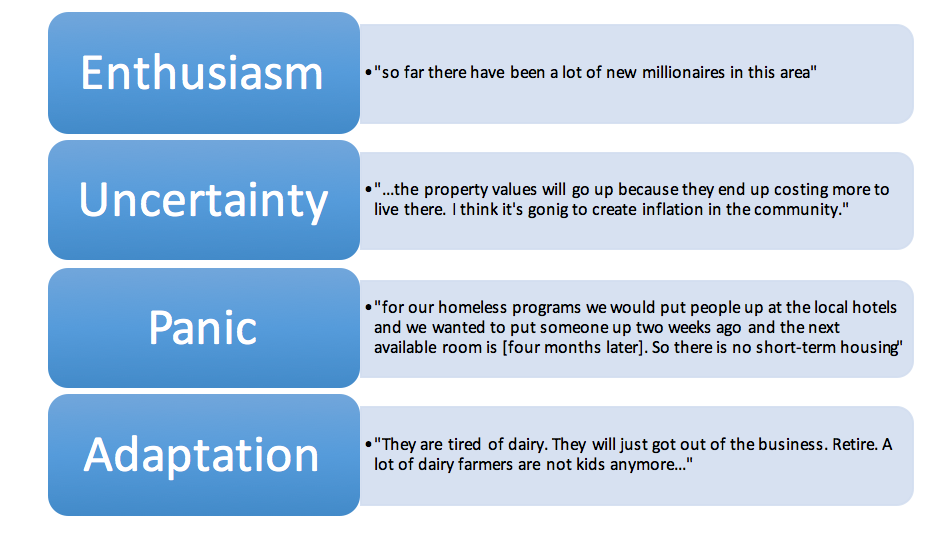
Research shows that the attitudes of residents of boomtowns generally progress through four stages:

Compiled by Grace Wildermuth
Residents may be enthusiastic as they consider the possible positive impacts (jobs, economic growth, etc.) that energy development could bring to their community. As development begins, however, their positive expectations may not be met as they discover unexpected negative side-effects or undesirable changes (environmental impacts, noise or odor, housing shortages, and rent increases). Panic may set in as residents fully realize the negative impacts that energy development has brought to their community. And finally, residents turn towards an attitude of adaptation as they grow accustomed to the new aspects of their community, both positive and negative.
Examples of each state from your reading:

Compiled by Grace Wildermuth
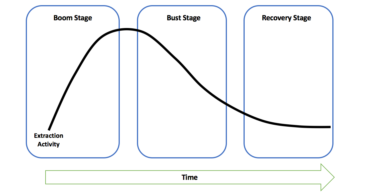
We can also look at boomtowns on the community level. Boomtown communities generally follow a boom-bust-recovery model (refer back to your notes from Activity 2). The figure below illustrates how the boomtown impact model predicts a community will move from the boom stage to the bust stage, and eventually the recovery stage over time.

Compiled by Grace Wildermuth
Boom stage
The ‘boom’ stage is characterized by a rapidly growing demand for a skilled labor force. Initially, rural communities are not able to supply the labor needed, resulting in rapid in-migration of workers and potentially their families and others to provide services to this population (Cortese & Jones, 1977; Albrecht, 1978). With a larger labor force, more money flows into the local economy; however, as demand for goods and services increases, inflation may ensue as well as stratification between those who can afford the goods and those who cannot (Jacquet, 2009).
Bust Stage
When the extracted resource becomes depleted or becomes less profitable, the employment opportunities offered by energy development begin to seep out of the community. Subsequently, outmigration occurs, decreasing revenue for local businesses and leaving an abundance of over produced infrastructure (Jacquet, 2009).
Recovery Stage
Some long-term research on boomtown communities has suggested a ‘recovery stage’ when community members, local leaders and businesses adapt to the environmental, social, and economic changes happening in their communities due to energy development.
A community’s progression from the boom to bust stages of this model are driven by the demand for the resource being developed, fluctuations in the products’ market price, changes and/or advancements in the extraction technology, new and evolving extraction processes or methods, and political conditions and/or decisions.
More recently, researchers have begun to modify the traditional boomtown impact model that examines a singular boom followed by a one-time bust. Instead, they believe, communities such as those in the Marcellus Shale region are likely to experience many mini-booms and mini-busts over the course of development. This new boomtown impact model suggests a different experience for communities and residents than the traditional boom-bust cycle (Jacquet & Kay 2014, Stedman et al 2012).

Compiled by Grace Wildermuth

Compiled by Grace Wildermuth
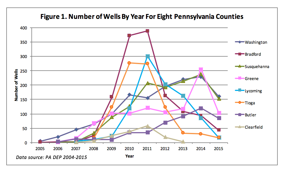
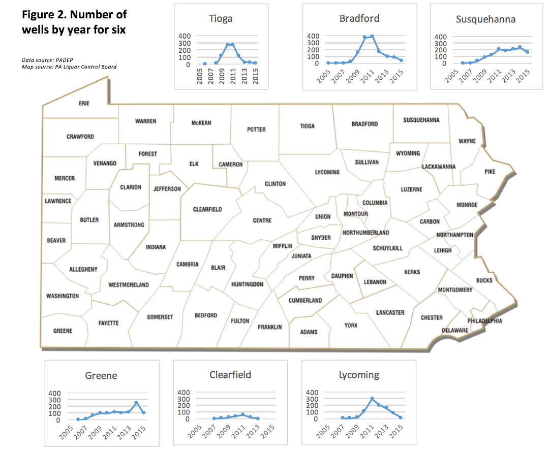
A new boomtown impact model is necessary to capture the effects of Marcellus Shale development. The wide geographic footprint and other characteristics of the resource, the industry’s strategic development plans, supply and demand of the resource, infrastructure development, and price fluctuation are just some of the factors that lead to a model that shows variation over space and time. Small scale “semi-busts and re-booms” (Jacquet and Kay, 2014) have occurred across Pennsylvania, as illustrated by the data above. Figure 1 displays the temporal differences in the number of wells by county. For example, note that as most counties were experiencing a downward trend or “semi-bust” in 2015, Greene County experienced a sudden increase, or boom, in number of wells. Figure 2 shows the spatial differences in the number of wells by county. Note, for example, that even though Tioga, Bradford, Susquehanna and Lycoming counties are located in close geographic proximity, they show substantial differences in development trends.
Additional Assumptions
Below are some additional assumptions of the traditional boomtown impact model, as well as explanations as to why the model may need to be adjusted to fit Marcellus Shale development:
Rural and isolated communities
The Marcellus Shale formation is expansive, and therefore stretches over many types of communities: rural and urban, isolated and with expansive transportation networks.
Small pockets of natural resources that would be extracted over a short period of time
The Marcellus Shale formation covers a very wide geographic area. Some areas may be more suitable for development under certain conditions or with certain technologies. Therefore, the industry may move around the area as conditions change, perhaps leading to mini-booms and mini-busts for each community.
Differences in land ownership affect ability of community to retain wealth
The majority of mineral rights in the Marcellus region are owned by private landowners, although not necessarily the person who owns the surface rights. Through leasing and royalties, money is transferred from the industry directly to those local residents who own mineral rights. The percentage of local landowners who own their mineral rights varies across the state, with areas having a long history of resource extraction (oil, gas, coal) more likely to have severed surface/subsurface rights. Further, some counties have large private or public (e.g., state forests) landowners. These patterns of surface and mineral rights ownership will affect how much leasing/royalty income is taken in by local residents.
Economic development and corporate behavior
The economic context within which Marcellus Shale Development is taking place is markedly different from that in the 1970s when the traditional boomtown model was put forth. There are different rules, protections, and permitting requirements in place. The initial rapid leasing or “land grab”, foreign investment, and continued production at low prices all lead to a different era of economic development and corporate behavior.


