2.1: Alfred Wegener’s Continental Drift Hypothesis
- Page ID
- 6846
\( \newcommand{\vecs}[1]{\overset { \scriptstyle \rightharpoonup} {\mathbf{#1}} } \)
\( \newcommand{\vecd}[1]{\overset{-\!-\!\rightharpoonup}{\vphantom{a}\smash {#1}}} \)
\( \newcommand{\id}{\mathrm{id}}\) \( \newcommand{\Span}{\mathrm{span}}\)
( \newcommand{\kernel}{\mathrm{null}\,}\) \( \newcommand{\range}{\mathrm{range}\,}\)
\( \newcommand{\RealPart}{\mathrm{Re}}\) \( \newcommand{\ImaginaryPart}{\mathrm{Im}}\)
\( \newcommand{\Argument}{\mathrm{Arg}}\) \( \newcommand{\norm}[1]{\| #1 \|}\)
\( \newcommand{\inner}[2]{\langle #1, #2 \rangle}\)
\( \newcommand{\Span}{\mathrm{span}}\)
\( \newcommand{\id}{\mathrm{id}}\)
\( \newcommand{\Span}{\mathrm{span}}\)
\( \newcommand{\kernel}{\mathrm{null}\,}\)
\( \newcommand{\range}{\mathrm{range}\,}\)
\( \newcommand{\RealPart}{\mathrm{Re}}\)
\( \newcommand{\ImaginaryPart}{\mathrm{Im}}\)
\( \newcommand{\Argument}{\mathrm{Arg}}\)
\( \newcommand{\norm}[1]{\| #1 \|}\)
\( \newcommand{\inner}[2]{\langle #1, #2 \rangle}\)
\( \newcommand{\Span}{\mathrm{span}}\) \( \newcommand{\AA}{\unicode[.8,0]{x212B}}\)
\( \newcommand{\vectorA}[1]{\vec{#1}} % arrow\)
\( \newcommand{\vectorAt}[1]{\vec{\text{#1}}} % arrow\)
\( \newcommand{\vectorB}[1]{\overset { \scriptstyle \rightharpoonup} {\mathbf{#1}} } \)
\( \newcommand{\vectorC}[1]{\textbf{#1}} \)
\( \newcommand{\vectorD}[1]{\overrightarrow{#1}} \)
\( \newcommand{\vectorDt}[1]{\overrightarrow{\text{#1}}} \)
\( \newcommand{\vectE}[1]{\overset{-\!-\!\rightharpoonup}{\vphantom{a}\smash{\mathbf {#1}}}} \)
\( \newcommand{\vecs}[1]{\overset { \scriptstyle \rightharpoonup} {\mathbf{#1}} } \)
\( \newcommand{\vecd}[1]{\overset{-\!-\!\rightharpoonup}{\vphantom{a}\smash {#1}}} \)
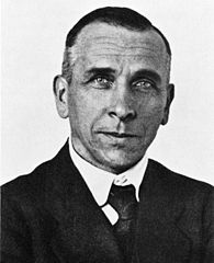
\(\newcommand{\avec}{\mathbf a}\) \(\newcommand{\bvec}{\mathbf b}\) \(\newcommand{\cvec}{\mathbf c}\) \(\newcommand{\dvec}{\mathbf d}\) \(\newcommand{\dtil}{\widetilde{\mathbf d}}\) \(\newcommand{\evec}{\mathbf e}\) \(\newcommand{\fvec}{\mathbf f}\) \(\newcommand{\nvec}{\mathbf n}\) \(\newcommand{\pvec}{\mathbf p}\) \(\newcommand{\qvec}{\mathbf q}\) \(\newcommand{\svec}{\mathbf s}\) \(\newcommand{\tvec}{\mathbf t}\) \(\newcommand{\uvec}{\mathbf u}\) \(\newcommand{\vvec}{\mathbf v}\) \(\newcommand{\wvec}{\mathbf w}\) \(\newcommand{\xvec}{\mathbf x}\) \(\newcommand{\yvec}{\mathbf y}\) \(\newcommand{\zvec}{\mathbf z}\) \(\newcommand{\rvec}{\mathbf r}\) \(\newcommand{\mvec}{\mathbf m}\) \(\newcommand{\zerovec}{\mathbf 0}\) \(\newcommand{\onevec}{\mathbf 1}\) \(\newcommand{\real}{\mathbb R}\) \(\newcommand{\twovec}[2]{\left[\begin{array}{r}#1 \\ #2 \end{array}\right]}\) \(\newcommand{\ctwovec}[2]{\left[\begin{array}{c}#1 \\ #2 \end{array}\right]}\) \(\newcommand{\threevec}[3]{\left[\begin{array}{r}#1 \\ #2 \\ #3 \end{array}\right]}\) \(\newcommand{\cthreevec}[3]{\left[\begin{array}{c}#1 \\ #2 \\ #3 \end{array}\right]}\) \(\newcommand{\fourvec}[4]{\left[\begin{array}{r}#1 \\ #2 \\ #3 \\ #4 \end{array}\right]}\) \(\newcommand{\cfourvec}[4]{\left[\begin{array}{c}#1 \\ #2 \\ #3 \\ #4 \end{array}\right]}\) \(\newcommand{\fivevec}[5]{\left[\begin{array}{r}#1 \\ #2 \\ #3 \\ #4 \\ #5 \\ \end{array}\right]}\) \(\newcommand{\cfivevec}[5]{\left[\begin{array}{c}#1 \\ #2 \\ #3 \\ #4 \\ #5 \\ \end{array}\right]}\) \(\newcommand{\mattwo}[4]{\left[\begin{array}{rr}#1 \amp #2 \\ #3 \amp #4 \\ \end{array}\right]}\) \(\newcommand{\laspan}[1]{\text{Span}\{#1\}}\) \(\newcommand{\bcal}{\cal B}\) \(\newcommand{\ccal}{\cal C}\) \(\newcommand{\scal}{\cal S}\) \(\newcommand{\wcal}{\cal W}\) \(\newcommand{\ecal}{\cal E}\) \(\newcommand{\coords}[2]{\left\{#1\right\}_{#2}}\) \(\newcommand{\gray}[1]{\color{gray}{#1}}\) \(\newcommand{\lgray}[1]{\color{lightgray}{#1}}\) \(\newcommand{\rank}{\operatorname{rank}}\) \(\newcommand{\row}{\text{Row}}\) \(\newcommand{\col}{\text{Col}}\) \(\renewcommand{\row}{\text{Row}}\) \(\newcommand{\nul}{\text{Nul}}\) \(\newcommand{\var}{\text{Var}}\) \(\newcommand{\corr}{\text{corr}}\) \(\newcommand{\len}[1]{\left|#1\right|}\) \(\newcommand{\bbar}{\overline{\bvec}}\) \(\newcommand{\bhat}{\widehat{\bvec}}\) \(\newcommand{\bperp}{\bvec^\perp}\) \(\newcommand{\xhat}{\widehat{\xvec}}\) \(\newcommand{\vhat}{\widehat{\vvec}}\) \(\newcommand{\uhat}{\widehat{\uvec}}\) \(\newcommand{\what}{\widehat{\wvec}}\) \(\newcommand{\Sighat}{\widehat{\Sigma}}\) \(\newcommand{\lt}{<}\) \(\newcommand{\gt}{>}\) \(\newcommand{\amp}{&}\) \(\definecolor{fillinmathshade}{gray}{0.9}\)Alfred Wegener (1880-1930) was a German scientist who specialized in meteorology and climatology. His knack for questioning accepted ideas started in 1910 when he disagreed with the explanation that the Bering Land Bridge was formed by isostasy and that similar land bridges once connected the continents [1]. After reviewing the scientific literature, he published a hypothesis stating the continents were originally connected and then drifted apart. While he did not have the precise mechanism worked out, his hypothesis was backed up by a long list of evidence.
Early Evidence for Continental Drift Hypothesis
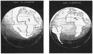
Wegener’s first piece of evidence was that the coastlines of some continents fit together like pieces of a jigsaw puzzle. People noticed the similarities in the coastlines of South America and Africa on the first world maps, and some suggested the continents had been ripped apart [3]. Antonio Snider-Pellegrini did preliminary work on continental separation and matching fossils in 1858.
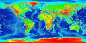
What Wegener did differently was synthesizing a large amount of data in one place. He used the true edges of the continents, based on the shapes of the continental shelves [4]. This resulted in a better fit than previous efforts that traced the existing coastlines [5].
![By Osvaldocangaspadilla (Own work) [Public domain], <a data-cke-saved-href="https://commons.wikimedia.org/wiki/File%3ASnider-Pellegrini_Wegener_fossil_map.svg" href="https://commons.wikimedia.org/wiki/File%3ASnider-Pellegrini_Wegener_fossil_map.svg" There are four different fossil organisms that connect South America, Africa, India, Antartica, and Australia.](http://opengeology.org/textbook/wp-content/uploads/2017/03/Wegener_fossil_map.svg_-300x231.png) via Wikimedia Commons" width="407px" height="313px" src="/@api/deki/files/8011/Wegener_fossil_map.svg_-300x231.png">
via Wikimedia Commons" width="407px" height="313px" src="/@api/deki/files/8011/Wegener_fossil_map.svg_-300x231.png">
Wegener also compiled evidence by comparing similar rocks, mountains, fossils, and glacial formations across oceans. For example, the fossils of the primitive aquatic reptile Mesosaurus were found on the separate coastlines of Africa and South America. Fossils of another reptile, Lystrosaurus, were found in Africa, India, and Antarctica. He pointed out these were land-dwelling creatures could not have swum across an entire ocean.
Opponents of continental drift insisted trans-oceanic land bridges allowed animals and plants to move between continents [6]. The land bridges eventually eroded away, leaving the continents permanently separated. The problem with this hypothesis is the improbability of a land bridge being tall and long enough to stretch across a broad, deep ocean.
More support for continental drift came from the puzzling evidence that glaciers once existed in normally very warm areas in southern Africa, India, Australia, and Arabia. These climate anomalies could not be explained by land bridges. Wegener found similar evidence when he discovered tropical plant fossils in the frozen region of the Arctic Circle. As Wegener collected more data, he realized the explanation that best fit all the climate, rock, and fossil observations involved moving continents.
Proposed Mechanism for Continental Drift
GFDL, CC-BY-SA-3.0 or CC BY-SA 2.5-2.0-1.0], via Wikimedia Commons" width="366px" height="275px" src="/@api/deki/files/8010/Convection-300x225.gif">
Figure \(\PageIndex{5}\): [Click to Animate] Animation of the basic idea of convection: an uneven heat source in a fluid causes rising material next to the heat and sinking material far from the heat.
Wegener’s work was considered a fringe science theory for his entire life. One of the biggest flaws in his hypothesis was the inability to provide a mechanism for how the continents moved. Obviously, the continents did not appear to move, and changing the conservative minds of the scientific community would require exceptional evidence that supported a credible mechanism. Other pro-continental drift followers used expansion, contraction, or even the moon’s origin to explain how the continents moved. Wegener used centrifugal forces and precession, but this model was proven wrong [7]. He also speculated about seafloor spreading, with hints of convection, but could not substantiate these proposals [8]. As it turns out, current scientific knowledge reveals convection is the major force in driving plate movements.
Development of Plate Tectonic Theory
![By NASA [Public domain], <a data-cke-saved-href="https://commons.wikimedia.org/wiki/File%3AGlobal_plate_motion_2008-04-17.jpg" href="https://commons.wikimedia.org/wiki/File%3AGlobal_plate_motion_2008-04-17.jpg" The map shows many data points all over the world.](http://opengeology.org/textbook/wp-content/uploads/2016/07/Global_plate_motion_2008-04-17-300x212.jpg) via Wikimedia Commons" width="357px" height="252px" src="/@api/deki/files/8019/Global_plate_motion_2008-04-17-300x212.jpg">
via Wikimedia Commons" width="357px" height="252px" src="/@api/deki/files/8019/Global_plate_motion_2008-04-17-300x212.jpg">
Wegener died in 1930 on an expedition in Greenland. Poorly respected in his lifetime, Wegener and his ideas about moving continents seemed destined to be lost in history as fringe science. However, in the 1950s, evidence started to trickle in that made continental drift a more viable idea. By the 1960s, scientists had amassed enough evidence to support the missing mechanism—namely, seafloor spreading—for Wegener’s hypothesis of continental drift to be accepted as the theory of plate tectonics. Ongoing GPS and earthquake data analyses continue to support this theory. The next section provides the pieces of evidence that helped transform one man’s wild notion into a scientific theory.
Mapping of the Ocean Floors
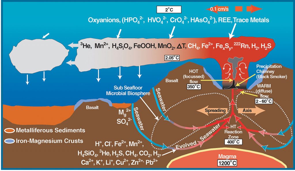
In 1947 researchers started using an adaptation of SONAR to map a region in the middle of the Atlantic Ocean with poorly-understood topographic and thermal properties [9]. Using this information, Bruce Heezen and Marie Tharp created the first detailed map of the ocean floor to reveal the Mid-Atlantic Ridge [10], a basaltic mountain range that spanned the length of the Atlantic Ocean, with rock chemistry and dimensions unlike the mountains found on the continents. Initially, scientists thought the ridge was part of a mechanism that explained the expanding Earth or ocean-basin growth hypotheses [11; 12]. In 1959, Harry Hess proposed the hypothesis of seafloor spreading – that the mid-ocean ridges represented tectonic plate factories, where a new oceanic plate was issuing from these long volcanic ridges. Scientists later included transform faults perpendicular to the ridges to better account for varying rates of movement between the newly formed plates [13]. When earthquake epicenters were discovered along the ridges, the idea that earthquakes were linked to plate movement took hold [14].
Seafloor sediment, measured by dredging and drilling, provided another clue. Scientists once believed sediment accumulated on the ocean floors over a very long time in a static environment. When some studies showed less sediment than expected, these results were initially used to argue against the continental movement [15; 16]. With more time, researchers discovered these thinner sediment layers were located close to mid-ocean ridges, indicating the ridges were younger than the surrounding ocean floor. This finding supported the idea that the seafloor was not fixed in one place [17].
Paleomagnetism
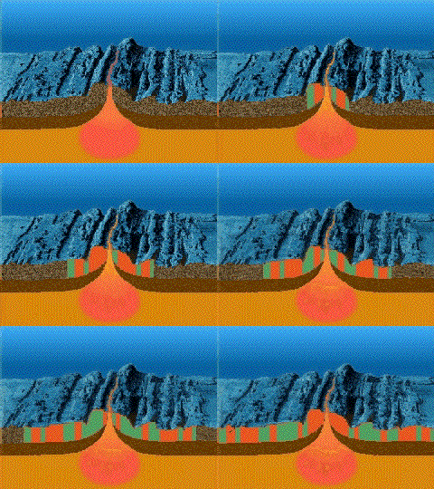
The seafloor was also mapped magnetically. Scientists had long known of strange magnetic anomalies that formed a striped pattern of symmetrical rows on both sides of mid-oceanic ridges. What made these features unusual was the north and south magnetic poles within each stripe was reversed in alternating rows [18]. By 1963, Harry Hess and other scientists used these magnetic reversal patterns to support their model for seafloor spreading [19] (see also Lawrence W. Morley [20]).
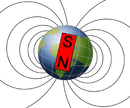
Paleomagnetism is the study of magnetic fields frozen within rocks, basically a fossilized compass. In fact, the first hard evidence to support plate motion came from paleomagnetism.
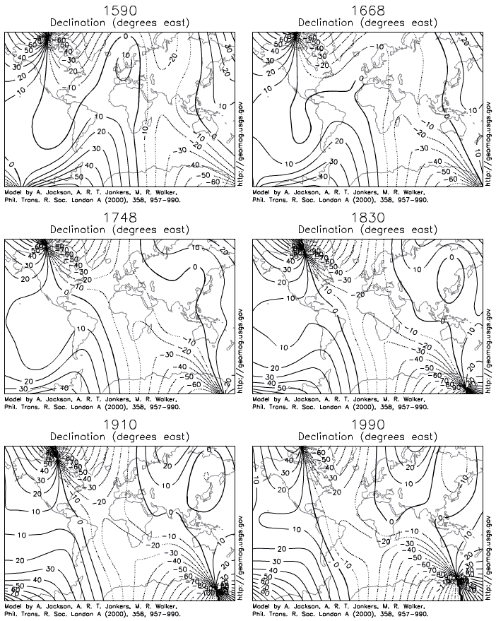
Igneous rocks containing magnetic minerals like magnetite typically provide the most useful data. In their liquid state as magma or lava, the magnetic poles of the minerals align themselves with the Earth’s magnetic field. When the rock cools and solidifies, this alignment is frozen into place, creating a permanent paleomagnetic record that includes magnetic inclination related to global latitude, and declination related to magnetic north.
Scientists had noticed for some time the alignment of magnetic north in many rocks was nowhere close to the earth’s current magnetic north. Some explained this as part of the normal movement of earth magnetic north pole. Eventually, scientists realized adding the idea of continental movement explained the data better than the pole movement alone [21].
Wadati-Benioff Zones
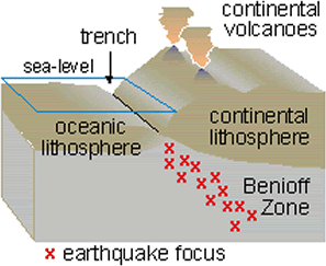
Around the same time mid-ocean ridges were being investigated, other scientists linked the creation of ocean trenches and island arcs to seismic activity and tectonic plate movement [22]. Several independent research groups recognized earthquake epicenters traced the shapes of oceanic plates sinking into the mantle. These deep earthquake zones congregated in planes that started near the surface around ocean trenches and angled beneath the continents and island arcs [23]. Today these earthquake zones called Wadati-Benioff zones.
 CC BY-SA 3.0 or GFDL], via Wikimedia Commons" width="217px" height="266px" src="/@api/deki/files/8026/John_Tuzo_Wilson_in_1992-244x300.jpg">
Based on the mounting evidence, the theory plate tectonics continued to take shape. J. Tuzo Wilson was the first scientist to put the entire picture together by proposing that the opening and closing of the ocean basins [24]. Before long, scientists proposed other models showing plates moving with respect to each other, with clear boundaries between them [25]. Others started piecing together complicated histories of tectonic plate movement [26]. The plate tectonic revolution had taken hold.
References
- 1. Fluegel, von H. W. Wegener-Ampferer-Schwinner. Ein Beitrag zur Geschichte der Geologie in Österreich. Mitt. Oesterr. Geol. Ges. 73, 237–254 (1980).
- 3. Bacon, F. & Montagu, B. The Works of Francis Bacon, Lord Chancellor of England: With a Life of the Author. (Parry & McMillan, 1848).
- 4. Drake, E. T. Alfred Wegener’s reconstruction of Pangea. Geology 4, 41–44 (1976).
- 5. Mantovani, R. Les fractures de l’écorce terrestre et la théorie de Laplace. Bull. Soc. Sc. et Arts Réunion 41–53 (1889).
- 6. Wells, H. G., Huxley, J. & Wells, G. P. The Science of Life. Philosophy 6, 506–507 (1931).
- 7. Scheidegger, A. E. Examination of the physics of theories of orogenesis. Geol. Soc. Am. Bull. 64, 127–150 (1953).
- 8. Jacoby, W. R. Modern concepts of Earth dynamics anticipated by Alfred Wegener in 1912. Geology 9, 25–27 (1981).
- 9. Tolstoy, I. & Ewing, M. North Atlantic hydrography and the Mid-Atlantic Ridge. Geol. Soc. Am. Bull. 60, 1527–1540 (1949).
- 10. Heezen, B. C., Tharp, M. & Ewing, M. The Floors of the Oceans I. The North Atlantic. Geological Society of America Special Papers 65, 1–126 (1959).
- 11. Heezen, B. C. The Rift in the Ocean Floor. Sci. Am. 203, 98–110 (1960).
- 12. Dietz, R. S. Continent and ocean basin evolution by spreading of the seafloor. Nature 190, 854–857 (1961).
- 13. Wilson, J. T. A new class of faults and their bearing on continental drift. Nature (1965).
- 14. Heezen, B. C. & Tharp, M. Tectonic Fabric of the Atlantic and Indian Oceans and Continental Drift. Philosophical Transactions of the Royal Society of London A: Mathematical, Physical and Engineering Sciences 258, 90–106 (1965).
- 15. Ewing, M., Ewing, J. I. & Talwani, M. Sediment distribution in the oceans: The Mid-Atlantic Ridge. Geol. Soc. Am. Bull. 75, 17–36 (1964).
- 16. Saito, T., Ewing, M. & Burckle, L. H. Tertiary sediment from the mid-atlantic ridge. Science 151, 1075–1079 (1966).
- 17. Ewing, M., Houtz, R. & Ewing, J. South Pacific sediment distribution. J. Geophys. Res. 74, 2477–2493 (1969).
- 18. Mason, R. G. A magnetic survey off the west coast of the United-States between latitudes 32-degrees-N and 36-degrees-N longitudes 121-degrees-W and 128-degrees-W. Geophysical Journal of the Royal Astronomical Society 1, 320 (1958).
- 19. Vine, F. J. & Matthews, D. H. Magnetic anomalies over oceanic ridges. Nature 199, 947–949 (1963).
- 20. Frankel, H. The Development, Reception, and Acceptance of the Vine-Matthews-Morley Hypothesis. Hist. Stud. Phys. Biol. Sci. 13, 1–39 (1982).
- 21. Irving, E. Palaeomagnetic and palaeoclimatological aspects of polar wandering. Geofis. pura appl. 33, 23–41 (1956).
- 22. Coats, R. R. Magma type and crustal structure in the Aleutian Arc. in The Crust of the Pacific Basin 92–109 (American Geophysical Union, 1962). doi:10.1029/GM006p0092
- 23. Wadati, K. On the activity of deep-focus earthquakes in the Japan Islands and neighbourhoods. Geophys. Mag. 8, 305–325 (1935).
- 24. Wilson, J. T. Did the Atlantic close and then re-open? (Nature, 1966).
- 25. McKenzie, D. P. & Parker, R. L. The North Pacific: an Example of Tectonics on a Sphere. Nature 216, 1276–1280 (1967).
- 26. Atwater, T. Implications of Plate Tectonics for the Cenozoic Tectonic Evolution of Western North America. Geol. Soc. Am. Bull. 81, 3513–3536 (1970).


