
8.3: Tides and Tidal Currents
- Page ID
- 13495
\( \newcommand{\vecs}[1]{\overset { \scriptstyle \rightharpoonup} {\mathbf{#1}} } \)
\( \newcommand{\vecd}[1]{\overset{-\!-\!\rightharpoonup}{\vphantom{a}\smash {#1}}} \)
\( \newcommand{\dsum}{\displaystyle\sum\limits} \)
\( \newcommand{\dint}{\displaystyle\int\limits} \)
\( \newcommand{\dlim}{\displaystyle\lim\limits} \)
\( \newcommand{\id}{\mathrm{id}}\) \( \newcommand{\Span}{\mathrm{span}}\)
( \newcommand{\kernel}{\mathrm{null}\,}\) \( \newcommand{\range}{\mathrm{range}\,}\)
\( \newcommand{\RealPart}{\mathrm{Re}}\) \( \newcommand{\ImaginaryPart}{\mathrm{Im}}\)
\( \newcommand{\Argument}{\mathrm{Arg}}\) \( \newcommand{\norm}[1]{\| #1 \|}\)
\( \newcommand{\inner}[2]{\langle #1, #2 \rangle}\)
\( \newcommand{\Span}{\mathrm{span}}\)
\( \newcommand{\id}{\mathrm{id}}\)
\( \newcommand{\Span}{\mathrm{span}}\)
\( \newcommand{\kernel}{\mathrm{null}\,}\)
\( \newcommand{\range}{\mathrm{range}\,}\)
\( \newcommand{\RealPart}{\mathrm{Re}}\)
\( \newcommand{\ImaginaryPart}{\mathrm{Im}}\)
\( \newcommand{\Argument}{\mathrm{Arg}}\)
\( \newcommand{\norm}[1]{\| #1 \|}\)
\( \newcommand{\inner}[2]{\langle #1, #2 \rangle}\)
\( \newcommand{\Span}{\mathrm{span}}\) \( \newcommand{\AA}{\unicode[.8,0]{x212B}}\)
\( \newcommand{\vectorA}[1]{\vec{#1}} % arrow\)
\( \newcommand{\vectorAt}[1]{\vec{\text{#1}}} % arrow\)
\( \newcommand{\vectorB}[1]{\overset { \scriptstyle \rightharpoonup} {\mathbf{#1}} } \)
\( \newcommand{\vectorC}[1]{\textbf{#1}} \)
\( \newcommand{\vectorD}[1]{\overrightarrow{#1}} \)
\( \newcommand{\vectorDt}[1]{\overrightarrow{\text{#1}}} \)
\( \newcommand{\vectE}[1]{\overset{-\!-\!\rightharpoonup}{\vphantom{a}\smash{\mathbf {#1}}}} \)
\( \newcommand{\vecs}[1]{\overset { \scriptstyle \rightharpoonup} {\mathbf{#1}} } \)
\(\newcommand{\longvect}{\overrightarrow}\)
\( \newcommand{\vecd}[1]{\overset{-\!-\!\rightharpoonup}{\vphantom{a}\smash {#1}}} \)
\(\newcommand{\avec}{\mathbf a}\) \(\newcommand{\bvec}{\mathbf b}\) \(\newcommand{\cvec}{\mathbf c}\) \(\newcommand{\dvec}{\mathbf d}\) \(\newcommand{\dtil}{\widetilde{\mathbf d}}\) \(\newcommand{\evec}{\mathbf e}\) \(\newcommand{\fvec}{\mathbf f}\) \(\newcommand{\nvec}{\mathbf n}\) \(\newcommand{\pvec}{\mathbf p}\) \(\newcommand{\qvec}{\mathbf q}\) \(\newcommand{\svec}{\mathbf s}\) \(\newcommand{\tvec}{\mathbf t}\) \(\newcommand{\uvec}{\mathbf u}\) \(\newcommand{\vvec}{\mathbf v}\) \(\newcommand{\wvec}{\mathbf w}\) \(\newcommand{\xvec}{\mathbf x}\) \(\newcommand{\yvec}{\mathbf y}\) \(\newcommand{\zvec}{\mathbf z}\) \(\newcommand{\rvec}{\mathbf r}\) \(\newcommand{\mvec}{\mathbf m}\) \(\newcommand{\zerovec}{\mathbf 0}\) \(\newcommand{\onevec}{\mathbf 1}\) \(\newcommand{\real}{\mathbb R}\) \(\newcommand{\twovec}[2]{\left[\begin{array}{r}#1 \\ #2 \end{array}\right]}\) \(\newcommand{\ctwovec}[2]{\left[\begin{array}{c}#1 \\ #2 \end{array}\right]}\) \(\newcommand{\threevec}[3]{\left[\begin{array}{r}#1 \\ #2 \\ #3 \end{array}\right]}\) \(\newcommand{\cthreevec}[3]{\left[\begin{array}{c}#1 \\ #2 \\ #3 \end{array}\right]}\) \(\newcommand{\fourvec}[4]{\left[\begin{array}{r}#1 \\ #2 \\ #3 \\ #4 \end{array}\right]}\) \(\newcommand{\cfourvec}[4]{\left[\begin{array}{c}#1 \\ #2 \\ #3 \\ #4 \end{array}\right]}\) \(\newcommand{\fivevec}[5]{\left[\begin{array}{r}#1 \\ #2 \\ #3 \\ #4 \\ #5 \\ \end{array}\right]}\) \(\newcommand{\cfivevec}[5]{\left[\begin{array}{c}#1 \\ #2 \\ #3 \\ #4 \\ #5 \\ \end{array}\right]}\) \(\newcommand{\mattwo}[4]{\left[\begin{array}{rr}#1 \amp #2 \\ #3 \amp #4 \\ \end{array}\right]}\) \(\newcommand{\laspan}[1]{\text{Span}\{#1\}}\) \(\newcommand{\bcal}{\cal B}\) \(\newcommand{\ccal}{\cal C}\) \(\newcommand{\scal}{\cal S}\) \(\newcommand{\wcal}{\cal W}\) \(\newcommand{\ecal}{\cal E}\) \(\newcommand{\coords}[2]{\left\{#1\right\}_{#2}}\) \(\newcommand{\gray}[1]{\color{gray}{#1}}\) \(\newcommand{\lgray}[1]{\color{lightgray}{#1}}\) \(\newcommand{\rank}{\operatorname{rank}}\) \(\newcommand{\row}{\text{Row}}\) \(\newcommand{\col}{\text{Col}}\) \(\renewcommand{\row}{\text{Row}}\) \(\newcommand{\nul}{\text{Nul}}\) \(\newcommand{\var}{\text{Var}}\) \(\newcommand{\corr}{\text{corr}}\) \(\newcommand{\len}[1]{\left|#1\right|}\) \(\newcommand{\bbar}{\overline{\bvec}}\) \(\newcommand{\bhat}{\widehat{\bvec}}\) \(\newcommand{\bperp}{\bvec^\perp}\) \(\newcommand{\xhat}{\widehat{\xvec}}\) \(\newcommand{\vhat}{\widehat{\vvec}}\) \(\newcommand{\uhat}{\widehat{\uvec}}\) \(\newcommand{\what}{\widehat{\wvec}}\) \(\newcommand{\Sighat}{\widehat{\Sigma}}\) \(\newcommand{\lt}{<}\) \(\newcommand{\gt}{>}\) \(\newcommand{\amp}{&}\) \(\definecolor{fillinmathshade}{gray}{0.9}\)Introduction
Go to any seacoast and build a tide gauge to obtain a record of sea level as a function of time (over a period of weeks or months) by somehow damping out or averaging over or filtering out the effects of waves on time scales of seconds and storms on time scales of days to weeks. What would you observe? In most places, you would find regular and systematic fluctuations in water level with dominant “periods” of about half a day or about one day, together with more subtle longer-term patterns on time scales of months and even years.
And if you then set up a similar tide gauge in a different place, you would find the same general effect (and the same frequency) but with differences in details of the shape of the time record, and also differences in timing of highs and lows.
As you all know, these effects you’re observing are the tides. It doesn’t take much brilliance on anybody’s part to relate the tides to the moon, because of identity of tidal periods and lunar periods. This was known in ancient times, and probably in even more distant prehistoric times. (It might trouble you, though, that the times of high and low tides are not coincident with the times when the moon is overhead; more on that later.)
Here’s the plan of action for this section on the tides:
- Forces involved in generating the tides, and the origin of the tidal bulge
- How the Earth’s rotation under the tidal bulges accounts for the observed tidal variations
- Forced-wave nature of the tides, which accounts for the phase lags observed
- Complicating effects needed to account for real tides: standing waves and Coriolis effects
- Tidal currents: periodic motions of the water in conjunction with the rise and fall of the tides
How Forces in the Earth–Moon System Cause the Tidal Bulge
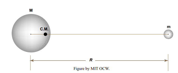
First, here are some comments on the Earth–Moon system, as an astronomical entity governed by the laws of mechanics. Usually one thinks of the Moon revolving about the Earth once in about each month. But it’s better to think of the Earth and the Moon as revolving around a single point, the center of mass of the Earth-Moon system. The Earth–Moon system together forms a mass unit, and it’s a well known principle in dynamics that the motions of this unit with respect to external forces can be analyzed in terms of an equal mass concentrated at the center of mass of the system. This is not the place for details, but here’s a homey example: throw a skinny dumbbell up in the air, and watch the way the center of mass follows a parabolic trajectory, just like a concentrated mass point, even though the dumbbell is twirling wildly. Because the Earth is much more massive than the Moon, the center of mass of the Earth–Moon system is actually inside the Earth, about 4600 km from the center (Figure 6-2)!
How do the Earth and the Moon stay in equilibrium? The rate of revolution of the two bodies about each other is such that the overall gravitational force of attraction is just in balance with the overall centrifugal force that tends to make the bodies fly apart from one another.
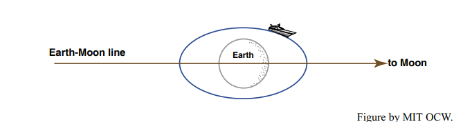
Given this overall balance, however, the local balance between centrifugal forces and gravitational forces differs from point to point within the Earth, depending upon the position the point relative to Earth–Moon axis. It’s this differing balance that causes the tides, by virtue of creating a bidirectional tidal bulge that draws the waters of the ocean out both in the direction of the Moon and in the direction away from the Moon, relative to directions normal to the Earth– Moon axis (Figure 6-3). (The solid Earth undergoes the same effect, as what are called earth tides, but because the solid Earth is a lot more rigid than the waters of the oceans the Earth tide is far smaller, only of the order of ten centimeters, than the ocean tide, which is a few meters, more or less.)
I imagine that the existence of this double-sided tidal bulge seems counterintuitive to you: why not just in the direction of the Moon? The following paragraphs attempt to provide a qualitative explanation, which itself will probably not seem immediately obvious to you; if you would like to see a more rigorous explanation, see the “advanced topic” section below.
The basic idea has to do with the relative magnitudes of two forces: the gravitational attraction of the Moon, and the centrifugal force on the Earth. As noted above, overall these two forces have to be in balance, or else the Earth– Moon system would not be in stable equilibrium with each other. The fundamental point is that, despite this overall balance, the relative magnitudes of the two forces vary from point to point within the Earth. The force of gravitational attraction is straightforward, but the centrifugal force needs some careful explanation. To help you understand it, try simulating the Earth–Moon system with your fists, as follows.
Make two fists. Hold the left fist pointing upward, and the right fist about a foot away, pointing downward. Your left fist represents the Earth, and your right fist represents the Moon. You can easily make your right fist revolve around your left fist in a circular orbit. But to simulate the motion of the Earth– Moon system, you need to move your left fist at the same time in a much smaller circular motion in the same sense of revolution, in such a way that the center of mass of the Earth–Moon system, which lies just inside your left fist, stays in the same place, relative to the floor below you. (It’s easier to do than to describe or to illustrate; I’ll demonstrate in class.)
Important: ignore the Earth’s rotation, because that’s not relevant to the origin of the tides. Concentrate on the circular revolution of the Earth (your left fist). Every point in your left fist is experiencing a centrifugal force, because of the circular motion, and that centrifugal force is the same at every point in your fist. Moreover, that centrifugal forces is always directed opposite to your right fist. (To understand that, you have to be doing the movements right.)
At the same time, every point in your left fist is experiencing a gravitational attraction from your right fist. That gravitational attraction is always directed toward your right fist. So at every point in your left fist there are two opposing forces, which are almost in balance. In contrast to the constant centrifugal force, the gravitational attraction of your right fist is slightly greater on the side of your left fist nearest your right fist and slightly smaller on the side of your left fist farthest from your right fist.
Now think about the relative magnitudes of the centrifugal force and the gravitational force. On the side nearest your right fist, the gravitational force is slightly larger than the centrifugal force, resulting in a net force directed outward from the surface of your left fist. On the side farthest from your right fist, the gravitational force is lightly smaller than the centrifugal force, also resulting in a net force outward from the surface of your left fist. These upward forces on opposite sides of your left fist are the forces that raise the tidal bulge on the two sides of the Earth!
I mentioned above that the Earth–Moon system is characterized by a balance between gravitational force and centrifugal force. By Newton’s law of universal gravitation, the gravitational force is
\[F=\frac{G m_{l} m_{2}}{r^{2}} \label{1}\]
where, given two bodies, F is the gravitational force of attraction between the two bodies, M1 is the mass of body 1, M2 is the mass of body 2, r is the distance between the centers of mass of the bodies, and G is the gravitational constant, equal to 6.667 x 10⁻⁸ cgs units. (Important note: this G is not the same as the acceleration of gravity g on Earth!). So, for the Earth–Moon system,
\[\text { centrifugal force }=\frac{G M m}{R^{2}} \label{2}\]
where M is the mass of the Earth, m is the mass of the moon, and R is the distance between the centers of mass of the Earth and the Moon.
But at any point on or in the Earth the local gravitational force and the local centrifugal force are not necessarily in balance. In terms of a unit mass located anywhere in the Earth, the centrifugal force (per unit mass) is the same everywhere, Gm/R2, found by dividing the overall centrifugal force by the mass of the Earth, but the gravitational force per unit mass varies from point to point because the distance from that point to the center of the Moon varies.
Why is the centrifugal force the same everywhere? (This is tricky to think about; at first thought, it seems as though it should vary from place to place.) I think the key here is to neglect the rotation of the Earth around its own axis; that’s a different centrifugal-force effect, not related in any way to analysis of the tides in terms of the revolution of the Earth and the Moon around their common center of mass.
If we assume that the orbits of the Earth and the Moon about their common center of mass are circles (actually they’re ellipses with very small eccentricity), a little thought should convince you that every point on the (nonrotating) Moon describes a circular path in space, and (important) the radii of all the circles are equal—although the circles are nonconcentric. And the same holds true for all points of the Earth, even though a nonrotating Earth revolves around a point actually located inside the Earth.
But how about the effect of the Earth’s rotation? That simply changes the equilibrium shape of the Earth to be a prolate spheroid instead of a sphere; it’s a matter of a balance between the “pancake” effect of the spin and the “glob” effect of the Earth’s own gravity field. The picture of tidal forces, based on considerations of gravitational versus centrifugal forces for a nonrotating Earth, is superimposed on this equilibrium shape.
Now think about the local balance of gravitational and centrifugal forces at two special points on the Earth: the point on the Earth’s surface that lies along the Earth–Moon axis on the side nearest the Moon (called the sublunar point), and the point on the Earth’s surface that lies along the Earth–Moon axis on the side farthest from the Moon (called the nadir point). Set up a coordinate system as shown in Figure 8-4. What I’m going to do is write the sum of the local gravitational force per unit mass and the local centrifugal force per unit mass at each of these special points.
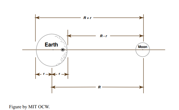
At the sublunar point the local gravitational force per unit mass is \(+Gm/(R - r)^2\), where \(R - r\) is the distance from the sublunar point to the center of mass of the Moon. The local centrifugal force is - \(Gm/R^2\), as discussed above; the minus sign is there because the centrifugal force acts in the direction opposite the gravitational force. So the sum of these two forces, which I’ll call \(F_T\), the net force per unit mass on Earth material located at the sublunar point, is
\[\begin{aligned}
F_{T} &=-\frac{G m}{R^{2}}+\frac{G m}{(R-r)^{2}} \\
&=\frac{-G m(R-r)^{2}+G m R^{2}}{R^{2}(R-r)^{2}} \\
&=G m\left[\frac{R^{2}-(R-r)^{2}}{R^{2}(R-r)^{2}}\right] \\
&=G m\left[\frac{2 r R-r^{2}}{R^{2}\left(R^{2}-2 r R+r^{2}\right)}\right]
\end{aligned} \label{3}\]
This looks formidable, but since \(r \ll R\), then \(r_2 \ll rR\) and \(rR \ll R_2\), so to a very close approximation
\[\begin{aligned}
F_{T} &=G m\left[\frac{2 R r}{R^{2}\left(R^{2}\right)}\right] \\
&=\frac{2 G m r}{R^{3}}
\end{aligned} \label{4}\]
On the opposite side of the Earth, at the nadir point, the same considerations on the net force per unit mass lead to
\[\begin{aligned}
F_{T} &=-\frac{G m}{R^{2}}+\frac{G m}{(R+r)^{2}} \\
&=G m\left[\frac{-(R+r)^{2}+R^{2}}{R^{2}(R+r)^{2}}\right] \\
&=G m\left[\frac{-2 r R-r^{2}}{R^{2}\left(R^{2}+2 r R+r^{2}\right)}\right] \\
&=G m\left[\frac{-2 r R}{R^{2}\left(R^{2}\right)}\right] \\
&=-\frac{2 G m r}{R^{3}}
\end{aligned} \label{5}\]
At this point we should expand our consideration from one dimension to two dimensions and think about all the points on the intersection of the Earth’s surface with any plane that passes through the Earth–Moon axis.
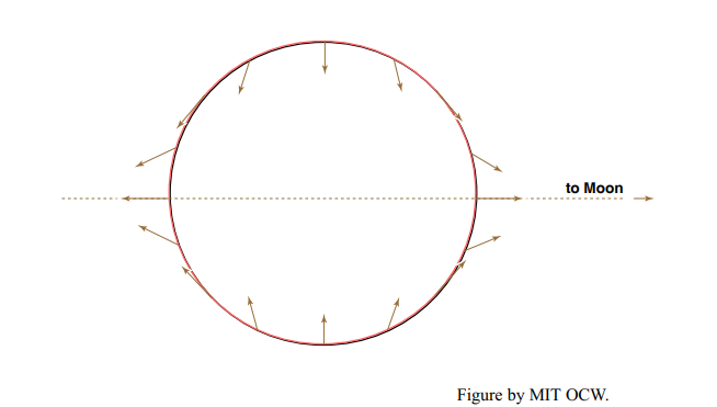
That’s more complicated mathematically, because we have an angle to worry about, but it’s straightforward. I won’t do it here. The result is shown qualitatively in Figure 8-6, which shows for a number of representative points the gravitational force, the centrifugal force, and the resultant of the two, and in Figure 8-7, which shows just the resultant.
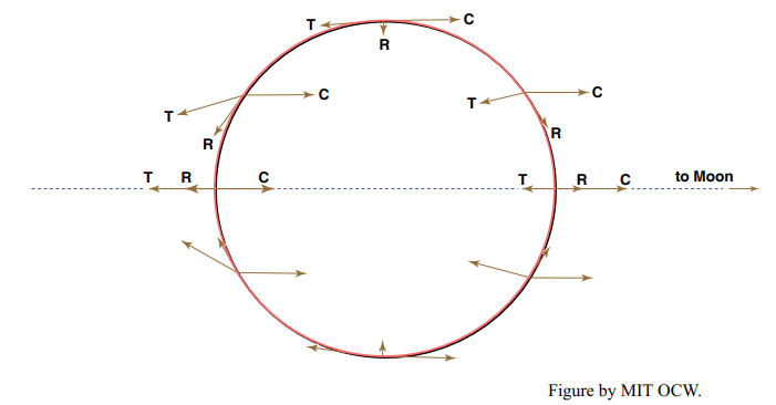
The forces shown in Figure 8-7 can themselves be resolved into components along the local vertical and the local horizontal. If you plug in some numbers, you would find that the local vertical component of FT is only about 10-7 that of the Earth’s gravitational pull on an object. So the vertical component of the net force is has a negligible effect on things like ocean water at the Earth’s surface. But the horizontal component of this net force is of about the same magnitude as the horizontal pressure-gradient forces that drive the water motions in the ocean. So the horizontal forces are important, and they can’t be ignored. They are what cause the tides.
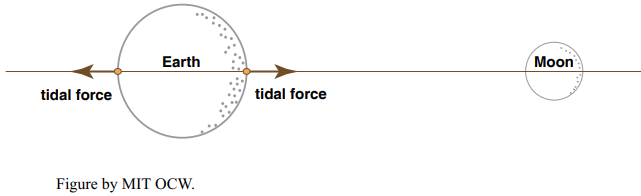
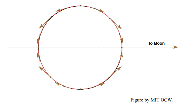
Figure 8-8 shows just the horizontal components of the net force FT at various points around the Earth. They’re zero at the sublunar and nadir points and at all points around the great circle that’s normal to the Earth–Moon axis, and they’re at a maximum around two small circles normal to the Earth–Moon axis and at 45° to that axis.
It’s these horizontal forces that cause the tides. They pile up ocean water in two symmetrical bulges at the sublunar point and the nadir point and lower the water level in the vicinity of the great circle normal to the Earth–Moon axis.
The Sun produces a tidal effect of the same kind as that of the Moon, but the effect is smaller. Although the Sun has far greater mass than the Moon, it’s also much farther away from the Earth. The tidal effect of the Sun is about 46% of that of the Moon. You can show this by forming the ratio
\[\frac{2 G m_{\text {moon }} r / R_{\text {moon }}^{3}}{2 G m_{\text {sun }} r / R_{\text {sun }}^{3}}\]
using the term on the right-hand side of Equation 4 or Equation 5 and substituting the appropriate values.
At this point you have to visualize that the Earth rotates on its axis under the tidal bulge, which, remember, is locked into position relative to the Moon. To you, the observer on the Earth, a tidal bulge seems to speed around the Earth twice a day, causing the rise and fall of the tides at your station. The period is the same as half the time it takes for the moon the reoccupy the meridian on successive days (24 hr 50.47 min, to be exact).
Some Complexities of the Equilibrium Tide
What I’ve presented above is basically what’s called the equilibrium theory of the tides. Newton laid the foundation by developing this concept, and the details were well worked out by over a hundred years ago. But this is really only the beginning of the story of the equilibrium tide, because we would have to get more deeply involved in analysis of the relative motions of the Earth, the Moon, and the Sun to take account of all the variations. Below are just two examples of such matters—but they are the two most important ones.
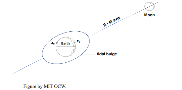
In general the Earth’s rotation axis is not perpendicular to the Earth– Moon axis. So when a point not on the Equator rotates under the two-ended tidal bulge the high tide at that point alternates between a higher high tide and a lower high tide (Figure 8-9). In Figure 8-9, a station at x1 has a higher high tide now, but about 12 hours later, when that same station experiences another high tide, that high tide is a lower high tide, because now the station is at x2, off the center of the tidal bulge. This is one cause of what’s called diurnal inequality, whereby one of the two semidiurnal tides is larger than the other at a given station.
A striking worldwide effect of the tides is an alternation between greater and smaller tidal ranges on a time period of one lunar month. Tides with the greater tidal ranges are called spring tides (no relation to the spring season of the year!), and tides with the smaller tidal ranges are called neap tides. The explanation of the spring–neap cycle is simple, and it has the side benefit of explaining also the phases of the Moon—something humankind in modern society has largely lost touch with, except for a swarm of boaters, smaller numbers of campers and fishermen, a rapidly shrinking group of old-fashioned gardeners and farmers who still insist on planting by the Moon, and a tiny band of scientists keeping knowledge alive.
In the course of one lunar month, the Moon makes one full revolution around the Earth. The Earth is at the same time revolving about the Sun, but it travels only a small fraction of a revolution in the time it takes for the Moon to go once around the Earth. Figure 8-10 shows the Moon at various positions around the Earth during one of its revolutions. The sense of rotation of the Earth around its own axis is shown also. The view in Figure 6-10 is perpendicular to the plane of revolution of the Earth around the Sun (called the plane of the ecliptic), and looking down onto the Northern Hemisphere of the Earth.
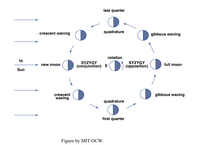
Twice during the month the Sun, the Earth, and the Moon are approximately in alignment. These are called syzygies (singular: syzygy). The syzygy for which the Moon is toward the Sun is called conjunction, and that for which the Moon is away from the Sun is called opposition. When the line between the Moon and the Earth makes a right angle with the line between the Sun and the Earth, the Moon is said to be in quadrature.
Obviously, the Sun and the Moon reinforce each other in their tidal effect at the time of syzygy, giving rise to spring tides, and they tend to cancel each other’s effects at the time of quadrature, giving rise to neap tides.
You can also see in Figure 8-10 the explanation for the phases of the Moon. At the time of conjunction, you can’t see the Moon; that’s called the new moon. At the time of opposition, you see the full moon. At the times of quadrature you see a half moon, officially called the first quarter and the last quarter. The full set of terms is given in Figure 8-10. If you think about it just a little, you can also see from Figure 8-10 why the Moon rises a little later each day throughout the lunar month; it’s because the sense of rotation of the Earth on its axis is the same as the sense of revolution of the Moon around the Earth, both being as shown in the figure.
There are many other such astronomical effects on the tides, having to do with
- the relative positions of the Earth, the Moon, and the Sun,
- the relative distance of the Moon from the Earth as a function of time during one lunar month, and
- the relative distance of the Sun from the Earth as a function of time during one year.
Accordingly, the tide varies complexly with time. These variations can be sorted out mathematically into what are called tidal constituents: regular periodic variations, with different amplitudes and periods, which are related directly or indirectly to the astronomical variations. These constituents are given names and code designations. Table 8-1 shows the most important ones. The principal lunar tide, M2, is the most important; it’s the one derived in the “advanced topic” section above.
Tides on the Real Earth
That something is disastrously wrong with the equilibrium theory of the tide should be apparent to anybody who makes intelligent observations of the tides: the time of high tide is not the same as the time when the Moon is at its highest point in the sky. There’s a time lag between the time the Moon is highest in the sky and the time of high tide. That time lag is called the lunitidal interval. It’s different at different points on the Earth, but it’s always the same at any given point.
The reason for this effect is tied up with the fact that the tide is a wave: it has two crests and two troughs around the world, and it moves as a progressive wave from east to west. As the tide wave passes, the water oscillates, just as when a much smaller wind-generated waves passes, as described in Chapter 1, but the water undergoes no net translation over one tidal cycle. (Actually that’s often not true in coastal environments with complex shoreline geometry and sea- bed topography, but it’s certainly true as a broad spatial average.)
In the terminology of Chapter 1, the tide wave is a grossly shallow- water wave: the ratio of water depth (a few kilometers) to wavelength (basically halfway around the Earth) is extremely small.

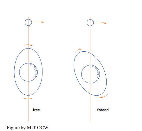
At this point you have to make a clear distinction between free waves and forced waves. A free wave propagates at a speed determined by its own wavelength and by the depth of water in which it’s propagating. A forced wave, on the other hand, is forced by external constraints to travel at some speed, slower or faster than its free-wave speed. The tide wave is clearly a forced wave, because it’s constrained, whether it likes to or not (and it doesn’t; see below), to travel around the Earth once a day. Whether such a forced wave lags behind its constraint or rides out in front of it depends on whether the ratio of the free-wave speed to the forced-wave speed is less than one or greater than one.
It’s well known from the theory of water waves that the speed of propagation of a shallow-water wave is equal to gh , where g is the acceleration of gravity and h is the water depth. You could easily compute from this that the free-wave speed of the tide wave is much less than the speed needed to get it around the Earth in one day. (Use 9.8 m/s2 for g, and assume a representative water depth of 4000 m in the oceans. The number of seconds in the lunar day of 24 hr 50.47 min is about 89,428.) So the tide wave lags behind the apparent motion of the Moon around the Earth (Figure 8-11).
We’re still not close to describing the true state of affairs in the real oceans. Only around the Southern Ocean, encircling a broad area in the Southern Hemisphere around Antarctica in the present configuration of the continents, can the tides do their thing as a wave that travels uninterruptedly all around the globe. All other areas of the oceans today are almost-closed basins, large or small, open only at their northern and/or southern ends. The critical question is: How do the tides behave in such basins?
The North Atlantic ocean basin is a good close-to-home example. If you ignore the minor effect of the narrow opening on the north into the Arctic Ocean, the North Atlantic is open only at its southern end. The basin feels a regularly rising and falling water level at its southern end. The effect of this rise and fall on the water levels and water motions in the basin is something that’s not quite within your everyday experience, but it’s something you could almost observe in your own bathtub. Here’s a very simple home experiment you can make to study the effects:
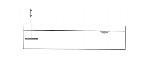
Cut a sheet of plywood into long strips and nail the strips together to form a simple long trough closed at both ends (Figure 8-12). On the bottom of one end of the trough, place a separate short board of wood that stretches almost from one side of the trough to the other. Nail a vertical stick to this little board so that you can move it up and down regularly, to oscillate the water level at that end of the tank. That simulates the periodic rise and fall of the tide wave at the southern end of the ocean basin.
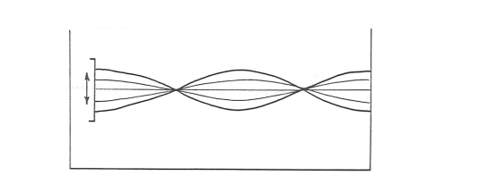
The up-and-down oscillation of the board at the end of your trough makes waves, and if your trough were endless you would just see a nice propagating train of waves, as described in Chapter 1. But the waves you make are reflected from the far wall of your trough. Those reflected waves travel back along the trough at the same speed as the oncoming waves, and they are of about the same amplitude (if you neglect the slight loss in energy when they’re reflected at the vertical wall). The result is a beautiful pattern of standing waves, with nodes where the water level stays the same and antinodes where the oscillation in water level is at its maximum (Figure 8-13). The number of nodes depends on the length of your tank and the period of the oscillation you impose on it. So although waves are actually moving in both directions, all you see is their sum, a standing wave.
I used to have a wall phone in my kitchen, with one of those long spiraling lines to the handset. During particularly boring phone calls, I played at jiggling my end of the wire up and down to make standing waves on the wire. The faster I jiggled the wire, the more nodes I got. This is closely analogous to the behavior of the water in your trough.
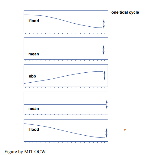
Figure 8-14 shows the standing wave in your trough as a time- sequence cartoon for the simple case of only one node, in the middle of the tank. Given the size of real ocean basins, and the speed and period of the tide wave, this is what you’re likely to find in the oceans. Note that the horizontal movement of the water is at its maximum at the nodes and is zero at the ends of the trough. This is just the kind of water motion observed in relatively long and narrow ocean basins.
The Bay of Fundy is a good example of tidal standing waves. You probably know that the tides at the head of the Bay of Fundy are the highest in the world. Why? Because the size and depth of the Bay of Fundy are just about such that its natural frequency is close to the natural period of oscillation of seiching. (A seiche is a periodic back-and-forth sloshing motion of water in an elongated lake or basin. Once a difference in water level between the two ends of the water body is set up—by the wind, for example—the sloshing continues until it dies out by friction.) The amplitude of the forced oscillation is well known to be greatest when the forcing period is close to the natural period; this condition is called resonance. You’ve all had lots of everyday experiences with resonance, whether you know it or not. Pumping on a swing is a good childhood example. Pushing your car in a rocking motion to get it unstuck on an icy road is a more grown-up example, as is sloshing the water in the roasting pan when you’re trying to scrub the pan in the sink.
But this still isn’t the end of the story! Unless the basin is very narrow, so that the water is constrained to move only back and forth, the Coriolis force has an important effect, unless you’re near the Equator. (See the following background section to learn something about the extremely important, but also extremely counterintuitive, Coriolis effect.) Figure 6-15 shows how the Coriolis force affects the water motions in the basin. Keep in mind that in the Northern Hemisphere the Coriolis force acts to the right of the direction of motion. So when the water is moving from the back end of the basin toward the front end, the Coriolis force banks it up against the left wall, until the downslope component of gravity, acting away from the left wall, balances the Coriolis force. Then, when the water is moving toward the back of the basin, the Coriolis force banks the water against the right wall. The result is a kind of circular sloshing motion that’s not easy to describe in a few words. This is called amphidromic motion.
In a large unobstructed indoor area (a gymnasium or a warehouse would be best, but a big room in your house would suffice), build a giant flat horizontal turntable—just a disk mounted at its center point on a vertical rotating shaft (Figure 8-16). You can rotate the whole disk at any desired constant rotation rate. It would be best if you painted the surface of the disk a flat black, the better to observe the motions of the brilliantly white marker spheres you’re going to roll around on the surface. To make things really exciting, be sure to coat the white marker spheres with a thick chalky coating of some sort that tracks off evenly onto the surface of the turntable as they roll about.
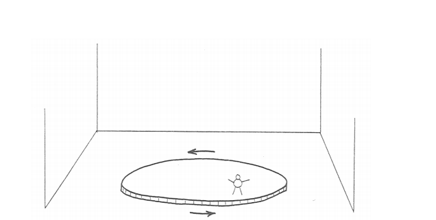
To do things right, you’re also going to need an observation perch above the turntable. This perch should be easily movable from place to place above the surface, but (and this is important) stationary relative to the floor of the room while in use. One of those mechanized cherry-picker seats, extending horizontally from the margin of the disk, would do nicely, if you can afford it.
Set the rotation rate, get into your perch, occupy a point just over the turntable, and roll one of your marked spheres onto the table, just as if you were at a bowling alley. Here’s the big question: What would the track of the sphere look like on the turntable? (You’re going to have to assume that the turntable exerts no substantial force on the rolling ball. That’s not really true, but the effects are small enough that you can safely ignore them for the purposes of this demonstration. If you don’t like that assumption, you can always imagine using a magic air-hockey puck that scoots frictionlessly over the turntable, leaving a powdery white trail behind it.)
The big jump that your powers of deduction or imagination have to take here is to see that the track left by the ball on the table would be curved (Figure 8- 17). (And, once you’re comfortable with that idea, it might naturally occur to you to think about whether that curved track is a circular arc. The answer turns out to be NO, although the reasons are a little too intricate to deal with at the moment.)
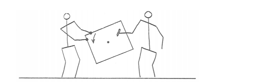
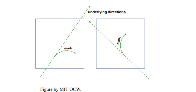
If you can’t afford the time and money to build the turntable, but you still want to get some useful results, here’s a much simpler and cheaper way of demonstrating the phenomenon (Figure 8-18). Pin a big piece of posterboard to the wall so that it can be rotated about its center point, and have an assistant stand to one side and rotate the posterboard in a hand-over-hand motion as steadily as possible. Stand in front of the posterboard with a marker pen, and draw a line on the posterboard in such a way that the tip of the pen is moving in uniform rectilinear motion relative to the underlying wall (that is, a straight line at constant speed). That’s tough to do, because you have to try to ignore the surface of the posterboard and the mark that’s coming out onto it and instead concentrate on the imaginary path of the pen point on the motionless wall behind. You would find (Figure 8-19) that no matter where you start on the posterboard, and no matter which direction you choose for your line, the mark on the posterboard is a curving arc!
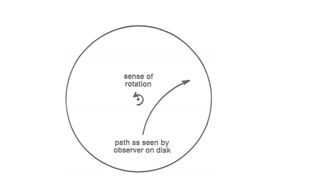
The next thing to do is have your assistant roll a marker sphere onto the turntable while you’re riding on the turntable. Watch the ball as it rolls and leaves its circular-arc track. It will look to you as though some mysterious sideways force is continuously acting on the ball normal to its path to push it off its course. Something seems to be wrong with Newton’s first law, which tells you that the ball should be moving in a straight line at constant speed. You know what the problem is, of course: the fictitious side force is an artifact of your observing the ball from the standpoint of the rotating turntable. If you reoccupied your perch and rolled a clean, chalkless ball onto the dimly lit black surface of the turntable, you’d see the ball roll in a nice straight line! The fictitious side force that seems to act on moving bodies in a rotating environment is called the Coriolis force, after the nineteenth-century French engineer–scientist Gaspard Gustave de Coriolis (1792–1843), who first studied the effect. And the apparent acceleration of the sphere (it’s a radial acceleration, not a tangential acceleration, in that only the direction changes, not the speed) is called the Coriolis acceleration. The entire effect is called the Coriolis effect.
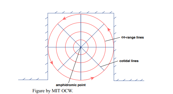
In basins like this (Figure 8-20), there’s some point in the center of the basin where the tidal change in water elevation is zero. That’s called an amphidromic point. Around the amphidromic point you can draw closed contours that give the loci of equal tidal range. These lines are called co-range lines. Finally, you can also draw spoke-like lines radiating outward from the amphidromic point toward the margins of the basin that show the locus of points at which the tide reaches a maximum at the same given time. These lines are called cotidal lines. A basin that has one amphidromic point with its associated cotidal lines and co-range lines is called an amphidromic system. Figure 8-21 shows the North Atlantic as an amphidromic system. The complex geometry of the bottom topography and shoreline trace makes the details of the amphidromic system irregular, but the essential features are clearly there.
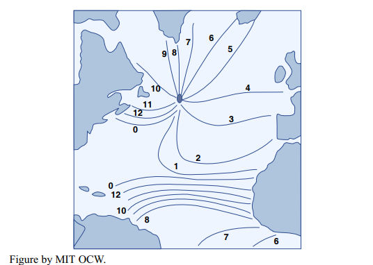
Large amphidromic systems can act as drivers or forcers for smaller amphidromic systems. Smaller basins like large gulfs or bays around the margins of a large ocean basin have their own amphidromic systems, which are forced by the periodic tidal rise and fall of water level at their mouths as the tide sweeps amphidromically around the larger basin. But whatever the size of the basin, the foregoing exposition serves to explain nicely the progressive difference in times of low tide and high tide along a given stretch of coastline. Figure 8-21 shows why the times of low and high tides get later and later from north to south along the east coast of North America.
Tidal Currents
Tidal currents are the horizontal water movements associated with the tidal rise and fall of the sea surface. If you occupy a station in the ocean, you observe not only a systematic change in water level but also a systematic change in current velocity.
The connection between tidal water-surface elevation and tidal- current velocity is an indirect one, though. Because of the complexity of the actual tidal wave, depending on where you are there can be different relationships between the tide and the tidal current, and there can even be places with tides but no tidal currents, or tidal currents but no tides. But this shouldn’t be too surprising, in light of our examination of standing tide waves in the preceding section. For the same reasons, there’s no direct relationship between the times of high and low tides and the times of slack water, when no tidal currents are running.
Another thing: you have to average over a time long enough compared to the tidal cycle to factor out currents caused by random effects like winds and storms—but with the added complication that there may be nonzero average currents at a locality, caused by currents of other kinds in the oceans. Also, don’t assume that the tidal currents themselves at a given locality have to average out to zero.
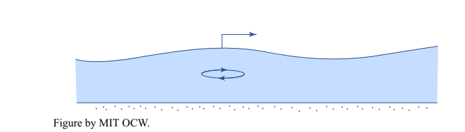
Why are there tidal currents? Tidal currents are simply the horizontal water motions associated with the passage of the tide wave, whatever the nature of that tide wave. Remember that tidal waves are very long compared to the water depth, so they are shallow-water waves. The water motion associated with such waves is a back-and-forth oscillation, actually an extremely flat ellipse, because the amplitude is so small relative to the wavelength (Figure 6-22). Even the sketch in Figure 6-22 has great vertical exaggeration, and also exaggeration of the length of the orbit.
Some definitions:
flood current: the current that runs while the tide is rising
ebb current: the current that runs while the tide is falling
slack water: the period of no tidal current while the tide reverses
(Note: the concept of slack water is relevant only to areas with nearly bidirectional tidal currents.)
Complications in tidal currents arise because there’s usually more than one progressive tidal wave, because of reflection, and commonly there are standing-wave systems as discussed above. So there’s no general relationship between high and low tide, on the one hand, and the time of slack water and the speed of the tidal currents, on the other hand. That relationship varies from area to area. The time of slack water may or may not be close to the times of high and low tides.
Another complication is that there’s no necessary relationship between the speed of the tidal current and the tidal range at a given place. In a very general way, of course, the speed of the tidal currents increases with the tidal range. But the speed of the tidal current is a matter of hydraulics, given the tidal range, and it depends on the volume of water moved versus the size of the passage through which the water has to move. For example, in the Gulf of Maine there’s a large tidal range but weak tidal currents, whereas in Nantucket Sound there’s a small tidal range but strong tidal currents. At a given station, however, the speed of the tidal currents is proportional to the tidal range, so currents are strongest during spring tides and weakest during neap tides.
How does one measure tidal currents? It’s more difficult than measuring the tidal range. Like any other measurement of current, it requires a station that’s fixed relative to the bottom, and a current meter of some kind. The picture of tidal currents is well known only for populated coastal areas.
What are the typical magnitudes of tidal currents? They’re highly variable. Strong tidal currents are 2–3 m/s at the surface (or 75–80% of this when depth-averaged). And 1–2 m/s tidal currents are very common. Currents like that can move a lot of sediment—if the sediment is there to move.
How does one represent tidal currents? The best way is to plot the tidal-current velocity vector as a function of time over a complete tidal cycle, with all the vectors having a common origin. That kind of plot is called a tidal-current rose. Figure 8-23 is an example from the Nantucket Shoals lightship. The following are some notes on Figure 8-23:
- The angular spacing of the vectors is not uniform, meaning that the turning of the current is not uniform in time.
- Low tide and high tide are not spaced equally in time.
- The maximum currents are not symmetrical in time.
- A floating object would make a closed traverse with the same shape (although not the same size!) as the curve connecting the tips of the vectors (and because the velocity vectors are turning clockwise, the object would move clockwise also).
- A current rose like that shown in Figure 8-23 is often approximately elliptical. If that’s the case, then it’s called a tidal ellipse.
- Current roses can be open, as in Figure 8-23, or more closed, as in Figure 8-24. As the current rose becomes flatter, the tidal currents become bidirectional tidal currents.