7.5: The Budget of Glaciers
- Page ID
- 13490
\( \newcommand{\vecs}[1]{\overset { \scriptstyle \rightharpoonup} {\mathbf{#1}} } \)
\( \newcommand{\vecd}[1]{\overset{-\!-\!\rightharpoonup}{\vphantom{a}\smash {#1}}} \)
\( \newcommand{\id}{\mathrm{id}}\) \( \newcommand{\Span}{\mathrm{span}}\)
( \newcommand{\kernel}{\mathrm{null}\,}\) \( \newcommand{\range}{\mathrm{range}\,}\)
\( \newcommand{\RealPart}{\mathrm{Re}}\) \( \newcommand{\ImaginaryPart}{\mathrm{Im}}\)
\( \newcommand{\Argument}{\mathrm{Arg}}\) \( \newcommand{\norm}[1]{\| #1 \|}\)
\( \newcommand{\inner}[2]{\langle #1, #2 \rangle}\)
\( \newcommand{\Span}{\mathrm{span}}\)
\( \newcommand{\id}{\mathrm{id}}\)
\( \newcommand{\Span}{\mathrm{span}}\)
\( \newcommand{\kernel}{\mathrm{null}\,}\)
\( \newcommand{\range}{\mathrm{range}\,}\)
\( \newcommand{\RealPart}{\mathrm{Re}}\)
\( \newcommand{\ImaginaryPart}{\mathrm{Im}}\)
\( \newcommand{\Argument}{\mathrm{Arg}}\)
\( \newcommand{\norm}[1]{\| #1 \|}\)
\( \newcommand{\inner}[2]{\langle #1, #2 \rangle}\)
\( \newcommand{\Span}{\mathrm{span}}\) \( \newcommand{\AA}{\unicode[.8,0]{x212B}}\)
\( \newcommand{\vectorA}[1]{\vec{#1}} % arrow\)
\( \newcommand{\vectorAt}[1]{\vec{\text{#1}}} % arrow\)
\( \newcommand{\vectorB}[1]{\overset { \scriptstyle \rightharpoonup} {\mathbf{#1}} } \)
\( \newcommand{\vectorC}[1]{\textbf{#1}} \)
\( \newcommand{\vectorD}[1]{\overrightarrow{#1}} \)
\( \newcommand{\vectorDt}[1]{\overrightarrow{\text{#1}}} \)
\( \newcommand{\vectE}[1]{\overset{-\!-\!\rightharpoonup}{\vphantom{a}\smash{\mathbf {#1}}}} \)
\( \newcommand{\vecs}[1]{\overset { \scriptstyle \rightharpoonup} {\mathbf{#1}} } \)
\( \newcommand{\vecd}[1]{\overset{-\!-\!\rightharpoonup}{\vphantom{a}\smash {#1}}} \)
\(\newcommand{\avec}{\mathbf a}\) \(\newcommand{\bvec}{\mathbf b}\) \(\newcommand{\cvec}{\mathbf c}\) \(\newcommand{\dvec}{\mathbf d}\) \(\newcommand{\dtil}{\widetilde{\mathbf d}}\) \(\newcommand{\evec}{\mathbf e}\) \(\newcommand{\fvec}{\mathbf f}\) \(\newcommand{\nvec}{\mathbf n}\) \(\newcommand{\pvec}{\mathbf p}\) \(\newcommand{\qvec}{\mathbf q}\) \(\newcommand{\svec}{\mathbf s}\) \(\newcommand{\tvec}{\mathbf t}\) \(\newcommand{\uvec}{\mathbf u}\) \(\newcommand{\vvec}{\mathbf v}\) \(\newcommand{\wvec}{\mathbf w}\) \(\newcommand{\xvec}{\mathbf x}\) \(\newcommand{\yvec}{\mathbf y}\) \(\newcommand{\zvec}{\mathbf z}\) \(\newcommand{\rvec}{\mathbf r}\) \(\newcommand{\mvec}{\mathbf m}\) \(\newcommand{\zerovec}{\mathbf 0}\) \(\newcommand{\onevec}{\mathbf 1}\) \(\newcommand{\real}{\mathbb R}\) \(\newcommand{\twovec}[2]{\left[\begin{array}{r}#1 \\ #2 \end{array}\right]}\) \(\newcommand{\ctwovec}[2]{\left[\begin{array}{c}#1 \\ #2 \end{array}\right]}\) \(\newcommand{\threevec}[3]{\left[\begin{array}{r}#1 \\ #2 \\ #3 \end{array}\right]}\) \(\newcommand{\cthreevec}[3]{\left[\begin{array}{c}#1 \\ #2 \\ #3 \end{array}\right]}\) \(\newcommand{\fourvec}[4]{\left[\begin{array}{r}#1 \\ #2 \\ #3 \\ #4 \end{array}\right]}\) \(\newcommand{\cfourvec}[4]{\left[\begin{array}{c}#1 \\ #2 \\ #3 \\ #4 \end{array}\right]}\) \(\newcommand{\fivevec}[5]{\left[\begin{array}{r}#1 \\ #2 \\ #3 \\ #4 \\ #5 \\ \end{array}\right]}\) \(\newcommand{\cfivevec}[5]{\left[\begin{array}{c}#1 \\ #2 \\ #3 \\ #4 \\ #5 \\ \end{array}\right]}\) \(\newcommand{\mattwo}[4]{\left[\begin{array}{rr}#1 \amp #2 \\ #3 \amp #4 \\ \end{array}\right]}\) \(\newcommand{\laspan}[1]{\text{Span}\{#1\}}\) \(\newcommand{\bcal}{\cal B}\) \(\newcommand{\ccal}{\cal C}\) \(\newcommand{\scal}{\cal S}\) \(\newcommand{\wcal}{\cal W}\) \(\newcommand{\ecal}{\cal E}\) \(\newcommand{\coords}[2]{\left\{#1\right\}_{#2}}\) \(\newcommand{\gray}[1]{\color{gray}{#1}}\) \(\newcommand{\lgray}[1]{\color{lightgray}{#1}}\) \(\newcommand{\rank}{\operatorname{rank}}\) \(\newcommand{\row}{\text{Row}}\) \(\newcommand{\col}{\text{Col}}\) \(\renewcommand{\row}{\text{Row}}\) \(\newcommand{\nul}{\text{Nul}}\) \(\newcommand{\var}{\text{Var}}\) \(\newcommand{\corr}{\text{corr}}\) \(\newcommand{\len}[1]{\left|#1\right|}\) \(\newcommand{\bbar}{\overline{\bvec}}\) \(\newcommand{\bhat}{\widehat{\bvec}}\) \(\newcommand{\bperp}{\bvec^\perp}\) \(\newcommand{\xhat}{\widehat{\xvec}}\) \(\newcommand{\vhat}{\widehat{\vvec}}\) \(\newcommand{\uhat}{\widehat{\uvec}}\) \(\newcommand{\what}{\widehat{\wvec}}\) \(\newcommand{\Sighat}{\widehat{\Sigma}}\) \(\newcommand{\lt}{<}\) \(\newcommand{\gt}{>}\) \(\newcommand{\amp}{&}\) \(\definecolor{fillinmathshade}{gray}{0.9}\)Economy vs. Regimen
First off, the term accumulation applies to all of the ways glacier ice mass is added to a glacier, and the term ablation applies to all of the ways glacier ice is removed from a glacier.
The term economy refers to the relative magnitude of accumulation and ablation. A glacier with accumulation greater than ablation over some period of time (much longer than just a single year) is said to have a positive economy, and gains ice volume with time. A glacier with accumulation less than ablation is said to have a negative economy, and loses ice volume with time. A glacier with a positive economy not only thickens but also extends its terminus in the downglacier direction. A glacier with a negative economy becomes thinner, and the terminus retreats upglacier.
The term regimen refers to the absolute values or magnitudes of accumulation and ablation, irrespective of their balance. A glacier with large values of accumulation and ablation is is said to have an active regimen, whereas a glacier with small values of both accumulation and ablation is said to have an inactive regimen. So there are four different combinations of economy and regimen.
Glacier Bookkeeping
Ice accumulates on a glacier by a variety of processes: snow (plus sleet and other solid precipitation), rain that gets frozen onto or into glacier, rime, frost, and avalanches. Snow is by far the most important of these.
Modes of ablation are melting (plus runoff and evaporation), sublimation, deflation by wind, and calving. The important ones are melting and, for glaciers that terminate in water, calving.
Occupy an observation point that’s fixed relative to the bedrock base or walls of the glacier, and consider any point on a the surface of the glacier.
Look at the vertical thickness of water (i.e., the height equivalent to solid ice) added to or lost at a point.
In glacier bookkeeping, an important concept is the balance year: the time between two successive dates with minimum mass of glacier ice at a given location on the glacier. Note: balance years are not necessarily 365 days, because the time of minimum ice mass depends upon the weather throughout the balance year, and the balance year can differ from point to point on the glacier.
Imagine plotting a graph showing the vertical ice-equivalent height added or subtracted as a function of time for a whole balance year (Figure 5-1). (Does the concept of “vertical ice-equivalent height” make sense to you? You have to convert accumulation and ablation into ice thickness.)
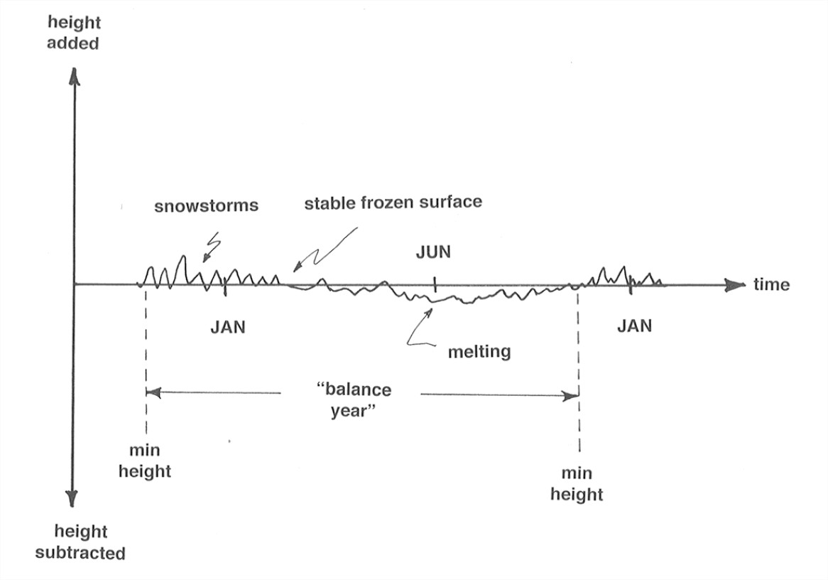
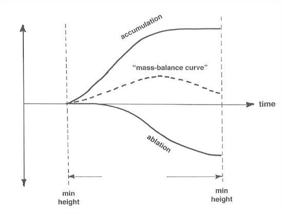
Now split the graph in Figure 1 into positive and negative parts (i.e., monotonically nonincreasing and monotonically nondecreasing), and then integrate (that is, keep track of a “running sum”) the two parts separately to get an accumulation curve and an ablation curve (Figure 7-2). The difference between the accumulation curve and the ablation curve is called the mass-balance curve. This curve is sort of the net change as you go along through the balance year. Don’t worry that it’s mostly above the horizontal axis; that’s only because we chose to work on the basis of minimum-height times as the starting and ending points of the balance year. The difference in elevation of the mass-balance curve and the horizontal axis at the end of the balance year is the net balance over the balance year, positive at this particular place and in this particular year.
BACKGROUND: INTEGRATION AND INTEGRALS
This is not the place for a full-scale calculus lesson, but for those of you who have not been exposed to the beauties of differential and integral calculus, here’s the concept of integration and integrals.
First, a few words about mathematical functions. You can think of a function as a magic box: you put a number into the box, and out comes a value that’s associated with that number. You’re probably more used to thinking of a function in strictly mathematical terms, in the form of an equation like y = x2: plug in a value for x, and the function gives you the value of y.
In mathematics, the process of integration involves a summation of the values of some function, as the value of the function varies over its range. If the function is defined only over a range of discrete values of the input variable (1, 2, 3, ... , let’s say), then the summation is simple and straightforward. All of you have done that. But how about when the function varies continuously over all values in the input variable, as, for example, the function y = x2 above? There’s a big conceptual leap involved here. The mathematical process by which the value of the function is summed continuously is called integration, and the value of the sum thus obtained is called an integral.
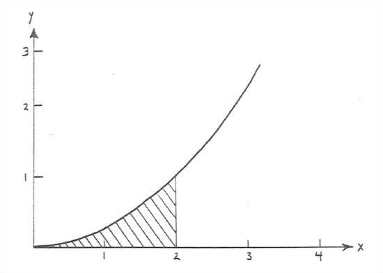
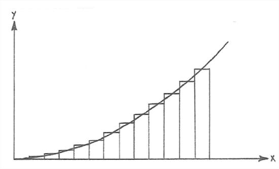
Obviously this is not the place either to develop the concept with mathematical rigor or to prescribe how to actually do integration. Here’s a simple example to show the results. Figure 7-3 shows the results of integrating the function y=x2 from x=0 to x=2. The curve in Figure 7-3 is that of the function y=x2, and the shaded area under the curve between x = 0 and x = 2 represents the value of the integral, which turns out to be exactly 2/3. Your common sense tells you it has to be a bit less than 1, which is what it would be if the function were the straight line y = x/2.
If somebody challenged you to find such an integral, without actually knowing how to do it mathematically, your clever mind might hit on the strategy of dividing up the x axis into a great many little segments and drawing rectangles with the value of y at the their tops, then figuring out the areas of all of the litle rectangles, and adding up all of those areas (Figure 7-4). That would be a good approximation to the integral you want to find. If you’re even sharper than that in such matters, you could imagine making the rectangles skinnier and skinnier, without limit. At that point you would be very close to the heart of the mathematical concept of integration!
The curves in Figures 7-1 and 7-2 differ from year to year at a point. Also, obviously they differ greatly from point to point: at points high on the glacier there’s a strongly positive net balance, maybe with no ablation all year, whereas low on the glacier there’s likely to be a strongly negative balance, with not much accumulation (presumably there’s always some) but lots of ablation.
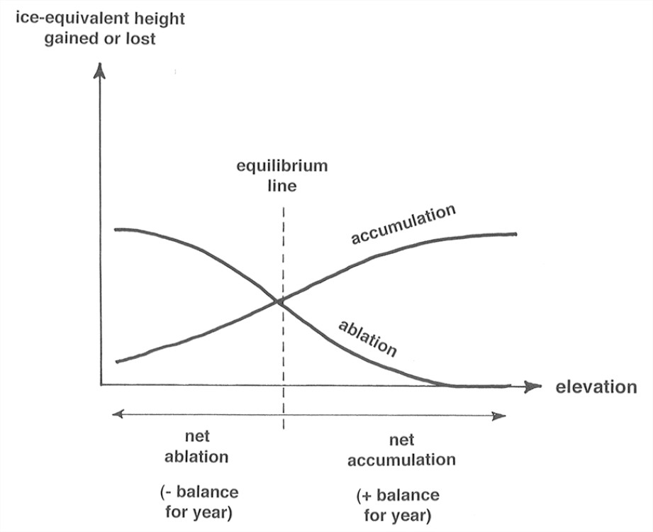
Figure 7-5 is a plot of ice-equivalent height gained by accumulation and lost by ablation as a function of elevation on a given glacier. In the right-hand part of the graph, high on the glacier, accumulation is greater than ablation, whereas in the left-hand part of the graph, low on the glacier, ablation is greater than accumulation. At a certain elevation the two curves intersect; this elevation is called the equilibrium line. Upglacier there’s still some of last year’s solid water (firn and glacier ice) left when new accumulation begins at the start of the new budget year; downglacier, all of last year’s snow melted before new accumulation starts. (Don’t worry about the areas under the curves; they don’t have to be equal, because they depend on the distribution of glacier area with elevation.)
Another thing you could do is integrate the accumulation and ablation curves in Figure 7-2 over the entire surface of the glacier to get the total accumulation and ablation. The result would look something like Figure 5-6. A little thought should convince you that glacier mass is unchanged through a given balance year if and only if Area 1 equals Area 2. If A1 < A2, the balance for that year is negative, and the glacier loses mass; if A1 > A2, the balance for that year is positive, and the glacier gains mass.
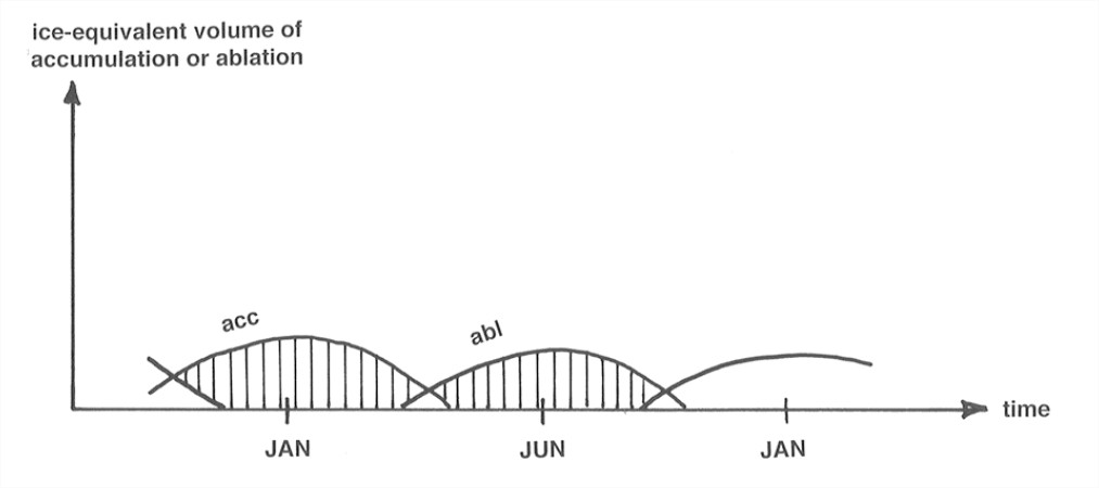
It is very difficult to obtain accumulation and ablation curves at points on a glacier. It’s easiest to measure (i.e., estimate) the net balance at many points in both the accumulation area and the ablation area and then integrate over the area of the glacier to find the net gain or loss of glacier mass for the given balance year. How? Dig pits down to last year’s snow in the accumulation area and then measure ablation at fixed stakes in the ablation area. (There’s some distortion involved, because of glacier movement.) Keeping track of accumulation and ablation as a function of time, as in Figure 7-4, is very time-consuming.
Features and relationships near the glacier surface around the equilibrium line are more complicated than I’ve indicated so far. To see this, imagine a survey from head to foot of the glacier at the end of summer melting season, to look at near-surface materials (Figure 7-7). Here are some comments on the various zones labeled in Figure 7-7.
- dry snow zone: no melting even in summer.
- percolation zone: some surface melting in summer. Water percolates down into snow at 0°C and refreezes, thereby warming the surrounding snow. Two characteristic forms of ice are deposited: ice layers or ice lenses, formed when water spreads out at some relatively impermeable horizon, and ice pipes or ice glands, formed by freezing of vertical water channels. The depth of saturation increases downglacier to the saturation line—the point where by the end of summer all of the snow deposited since the end of the previous summer has been saturated.
- soaked zone: by the end of the summer, all the current year’s snow has been saturated and raised to 0°C. Some meltwater also percolates into deeper layers.
- superimposed-ice zone: in the lower part of the soaked zone, at lower elevations, there’s so much meltwater that ice layers and patches among the firn merge to form a continuous mass of ice, called superimposed ice. Summer melting exposes this ice. The exposed part that remains at the end of the melting season is called the superimposed-ice zone. The firn line (the boundary between the current year’s snow and the newer ice) is easy to find.
- ablation zone: the zone below which all of the firn and superimposed ice from the current year has been melted away, to expose older ice.
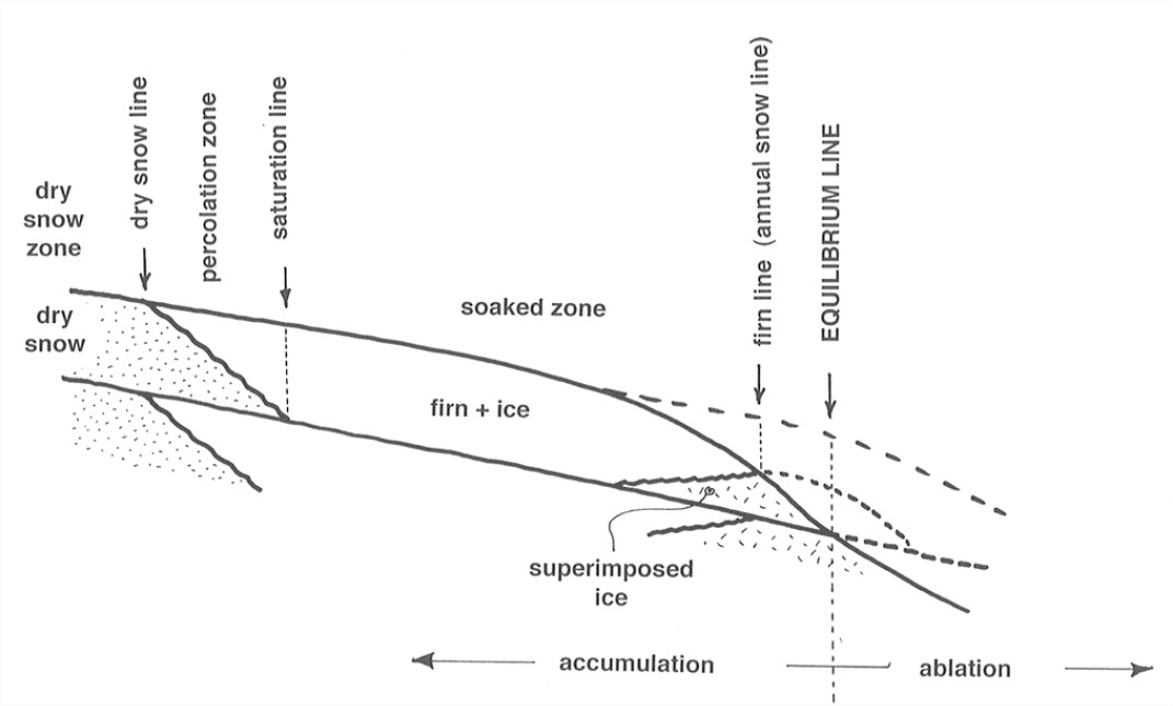
This is all highly idealized. Most glaciers don’t show all the zones, or at least not every season. The dry snow zone may be absent; melting eliminates all the superimposed ice if the net balance is negative; and the relative importance of evaporation and percolation varies. In a series of negative years, one can often see several “firn lines” or “firn edges” if development of superimposed ice is not important (Figure 7-8).
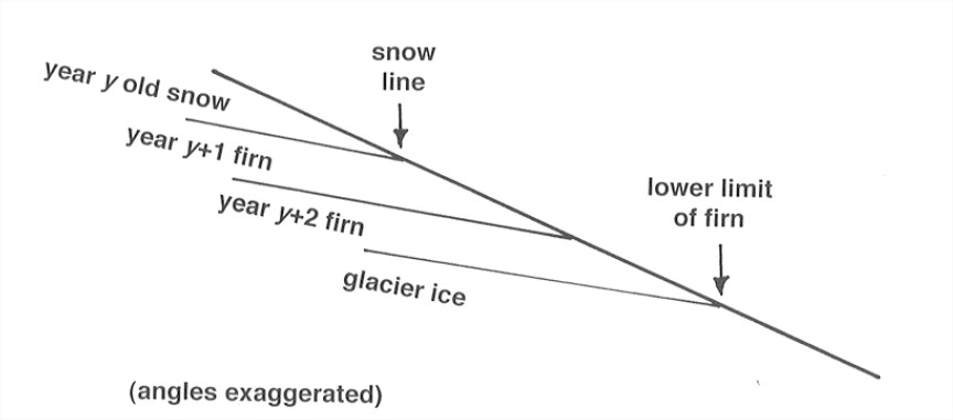
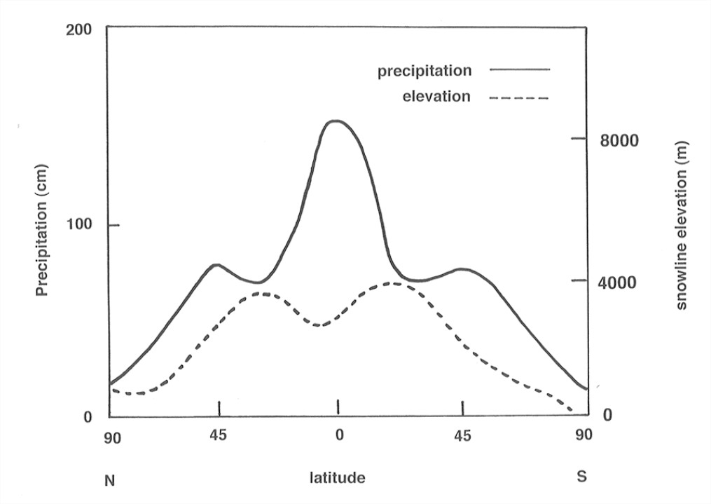
A concept closely related to the equilibrium line is the annual snowline: the lower limit of current year’s snow on the glacier surface. What are the controls on the snowline? Mainly winter precipitation and summer temperature. The annual snowline is the local manifestation of what’s called the regional snowline: a band with a width up to a couple of hundred meters in elevation in which the local snowline lies on regional scale (This band is patchy locally but very consistent regionally.) Figure 7-9 shows the average position of the regional snowline as a function of latitude, as well as the average precipitation.
