6.5: The Vertical Temperature Structure of Bath Water
- Page ID
- 13484
\( \newcommand{\vecs}[1]{\overset { \scriptstyle \rightharpoonup} {\mathbf{#1}} } \)
\( \newcommand{\vecd}[1]{\overset{-\!-\!\rightharpoonup}{\vphantom{a}\smash {#1}}} \)
\( \newcommand{\id}{\mathrm{id}}\) \( \newcommand{\Span}{\mathrm{span}}\)
( \newcommand{\kernel}{\mathrm{null}\,}\) \( \newcommand{\range}{\mathrm{range}\,}\)
\( \newcommand{\RealPart}{\mathrm{Re}}\) \( \newcommand{\ImaginaryPart}{\mathrm{Im}}\)
\( \newcommand{\Argument}{\mathrm{Arg}}\) \( \newcommand{\norm}[1]{\| #1 \|}\)
\( \newcommand{\inner}[2]{\langle #1, #2 \rangle}\)
\( \newcommand{\Span}{\mathrm{span}}\)
\( \newcommand{\id}{\mathrm{id}}\)
\( \newcommand{\Span}{\mathrm{span}}\)
\( \newcommand{\kernel}{\mathrm{null}\,}\)
\( \newcommand{\range}{\mathrm{range}\,}\)
\( \newcommand{\RealPart}{\mathrm{Re}}\)
\( \newcommand{\ImaginaryPart}{\mathrm{Im}}\)
\( \newcommand{\Argument}{\mathrm{Arg}}\)
\( \newcommand{\norm}[1]{\| #1 \|}\)
\( \newcommand{\inner}[2]{\langle #1, #2 \rangle}\)
\( \newcommand{\Span}{\mathrm{span}}\) \( \newcommand{\AA}{\unicode[.8,0]{x212B}}\)
\( \newcommand{\vectorA}[1]{\vec{#1}} % arrow\)
\( \newcommand{\vectorAt}[1]{\vec{\text{#1}}} % arrow\)
\( \newcommand{\vectorB}[1]{\overset { \scriptstyle \rightharpoonup} {\mathbf{#1}} } \)
\( \newcommand{\vectorC}[1]{\textbf{#1}} \)
\( \newcommand{\vectorD}[1]{\overrightarrow{#1}} \)
\( \newcommand{\vectorDt}[1]{\overrightarrow{\text{#1}}} \)
\( \newcommand{\vectE}[1]{\overset{-\!-\!\rightharpoonup}{\vphantom{a}\smash{\mathbf {#1}}}} \)
\( \newcommand{\vecs}[1]{\overset { \scriptstyle \rightharpoonup} {\mathbf{#1}} } \)
\( \newcommand{\vecd}[1]{\overset{-\!-\!\rightharpoonup}{\vphantom{a}\smash {#1}}} \)
\(\newcommand{\avec}{\mathbf a}\) \(\newcommand{\bvec}{\mathbf b}\) \(\newcommand{\cvec}{\mathbf c}\) \(\newcommand{\dvec}{\mathbf d}\) \(\newcommand{\dtil}{\widetilde{\mathbf d}}\) \(\newcommand{\evec}{\mathbf e}\) \(\newcommand{\fvec}{\mathbf f}\) \(\newcommand{\nvec}{\mathbf n}\) \(\newcommand{\pvec}{\mathbf p}\) \(\newcommand{\qvec}{\mathbf q}\) \(\newcommand{\svec}{\mathbf s}\) \(\newcommand{\tvec}{\mathbf t}\) \(\newcommand{\uvec}{\mathbf u}\) \(\newcommand{\vvec}{\mathbf v}\) \(\newcommand{\wvec}{\mathbf w}\) \(\newcommand{\xvec}{\mathbf x}\) \(\newcommand{\yvec}{\mathbf y}\) \(\newcommand{\zvec}{\mathbf z}\) \(\newcommand{\rvec}{\mathbf r}\) \(\newcommand{\mvec}{\mathbf m}\) \(\newcommand{\zerovec}{\mathbf 0}\) \(\newcommand{\onevec}{\mathbf 1}\) \(\newcommand{\real}{\mathbb R}\) \(\newcommand{\twovec}[2]{\left[\begin{array}{r}#1 \\ #2 \end{array}\right]}\) \(\newcommand{\ctwovec}[2]{\left[\begin{array}{c}#1 \\ #2 \end{array}\right]}\) \(\newcommand{\threevec}[3]{\left[\begin{array}{r}#1 \\ #2 \\ #3 \end{array}\right]}\) \(\newcommand{\cthreevec}[3]{\left[\begin{array}{c}#1 \\ #2 \\ #3 \end{array}\right]}\) \(\newcommand{\fourvec}[4]{\left[\begin{array}{r}#1 \\ #2 \\ #3 \\ #4 \end{array}\right]}\) \(\newcommand{\cfourvec}[4]{\left[\begin{array}{c}#1 \\ #2 \\ #3 \\ #4 \end{array}\right]}\) \(\newcommand{\fivevec}[5]{\left[\begin{array}{r}#1 \\ #2 \\ #3 \\ #4 \\ #5 \\ \end{array}\right]}\) \(\newcommand{\cfivevec}[5]{\left[\begin{array}{c}#1 \\ #2 \\ #3 \\ #4 \\ #5 \\ \end{array}\right]}\) \(\newcommand{\mattwo}[4]{\left[\begin{array}{rr}#1 \amp #2 \\ #3 \amp #4 \\ \end{array}\right]}\) \(\newcommand{\laspan}[1]{\text{Span}\{#1\}}\) \(\newcommand{\bcal}{\cal B}\) \(\newcommand{\ccal}{\cal C}\) \(\newcommand{\scal}{\cal S}\) \(\newcommand{\wcal}{\cal W}\) \(\newcommand{\ecal}{\cal E}\) \(\newcommand{\coords}[2]{\left\{#1\right\}_{#2}}\) \(\newcommand{\gray}[1]{\color{gray}{#1}}\) \(\newcommand{\lgray}[1]{\color{lightgray}{#1}}\) \(\newcommand{\rank}{\operatorname{rank}}\) \(\newcommand{\row}{\text{Row}}\) \(\newcommand{\col}{\text{Col}}\) \(\renewcommand{\row}{\text{Row}}\) \(\newcommand{\nul}{\text{Nul}}\) \(\newcommand{\var}{\text{Var}}\) \(\newcommand{\corr}{\text{corr}}\) \(\newcommand{\len}[1]{\left|#1\right|}\) \(\newcommand{\bbar}{\overline{\bvec}}\) \(\newcommand{\bhat}{\widehat{\bvec}}\) \(\newcommand{\bperp}{\bvec^\perp}\) \(\newcommand{\xhat}{\widehat{\xvec}}\) \(\newcommand{\vhat}{\widehat{\vvec}}\) \(\newcommand{\uhat}{\widehat{\uvec}}\) \(\newcommand{\what}{\widehat{\wvec}}\) \(\newcommand{\Sighat}{\widehat{\Sigma}}\) \(\newcommand{\lt}{<}\) \(\newcommand{\gt}{>}\) \(\newcommand{\amp}{&}\) \(\definecolor{fillinmathshade}{gray}{0.9}\)The vertical temperature structure of lakes is a surprisingly intricate matter, and one that’s more important than would seem at first thought. Remember that the density of water varies significantly with temperature, so if there’s exchange of heat between the lake and its environment, giving rise to temperature differences, buoyancy forces will cause motions of the lake water until a gravitationally stable arrangement is reached, with less dense water overlying more dense water. What makes these processes interestingly complex is the strange density maximum at 4°C, noted back in Chapter 1.
In one sense, the water in your bathtub is a good model of a small lake. Think about the temperature and density structure of your bath. First of all, here are the two obvious scenarios for how you draw your bath:
- First you run water that’s too cold, and then, to make it warmer, you run water that’s too hot (or vice versa). Then you swash it all around for a few seconds to wind up with a nice homogeneous well mixed bath at the desired temperature.
- You run it in all at the same temperature and then simply turn the tap off.
In both of these scenarios, if you measured the temperature with a little thermometer you’d find very close to the same temperature at all points. If you stuck in your little cream whipper coated with slowly soluble dye and beat the water, you’d generate a lot of turbulence and also set up a complicated circulation pattern through the entire bath, and the dye would rapidly become mixed uniformly throughout the bath.
You might think that the uniformly mixed situation described above is the normal situation in lakes, but it isn’t. To illustrate, here’s another bathtub scenario. First you put in hot water and then cold water, or vice versa, and then the phone rings and you don’t get a chance to mix them. When you come back to the bathtub you measure the vertical temperature profile. You’d find that the temperature is somewhat lower near the bottom than near the water surface (Figure 4-4). This temperature difference from bottom to top depends partly on the original temperature difference between the cold water and the hot water you used, but just as importantly on how fast you filled the tub. The stronger the water jet hitting the water surface, the greater the mixing between cold water and hot water.
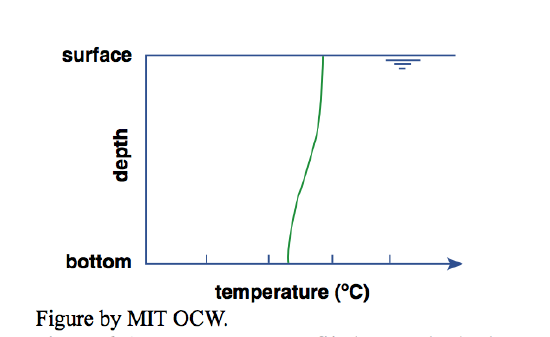
Why the temperature difference from bottom to top? Because cold water is denser than the hot water (provided that its temperature is above 4°C), so it tends to stay at the bottom (if you ran the cold water first) or find its way to the bottom (if you ran the hot water first). The only reason you don’t end up with a perfectly stratified situation, with all the original cold water as a lower layer and all the original hot water as an upper layer, is the mixing occasioned by the jet from the faucet as the jet impinges on the water surface during filling.
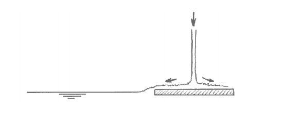
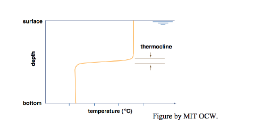
With a little extra effort you can indeed set up an almost perfectly two-layer temperature-stratified bath. You get the best results by filling first with cold water and then with hot water, and by letting the water jet fall on a spreading plate that floats on the surface (Figure 6-5). The purpose of the spreading plate is to break the momentum of the downward jet, so that the warm water flows slowly off the plate horizontally and has no chance to mix with the cold layer below. That leads to two nearly homogeneous layers, cold below and hot above, separated by a thin zone of very sharp temperature change (effectively a temperature discontinuity), called a thermocline (Figure 6-6). In real lakes, the thermocline is also called the metalimnion; the zone above is called the epilimnion, and the zone below is called the hypolimnion.
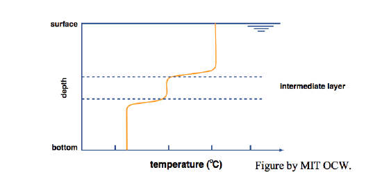
Now if you put in your little dye-coated beater, what would you see? If you put the beater in either the upper (hot) or the lower (cold) layer, you’d produce a lot of turbulence in that layer, but the other layer would be little affected: each layer acts largely independently of the other (Figure 6-7). If, however, you put the beater at the interface, you’d mix some of the hot and cold together to produce water with intermediate density and temperature, and that intermediate water would drift out laterally to form a new and easily recognizable intermediate layer (Figure 6-8).
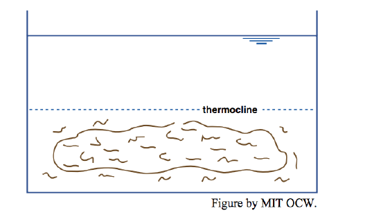
What’s going on here is that in arranging a cold layer below and a hot layer above you’ve produced a gravitationally stable stratification, and it takes work (literally, in the sense of physics—force times distance) to mix the waters of the two layers. The motions produced when the beater was in just one layer weren’t enough to disrupt the stratification. You’d need a more powerful mixer to break down the stable density stratification.
Here are a few other instructive things you could do in your bathtub to gain some insights into the thermal regime of lakes:
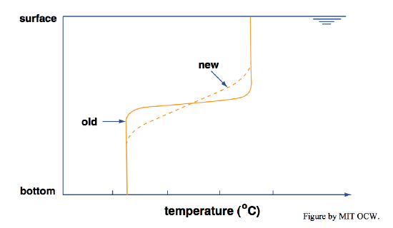
• Line your bathtub the best you can with a coating of thermal insulation, including a floating insulating lid. In this way you eliminate all possibility of changing the temperature and therefore the density of the bath water by exchange of heat with the environment. Start with a thermally stratified bath, as above, and then come back hours later and re-measure the vertical temperature profile. You’d find that the thermocline has thickened (Figure 6-9). Why? By conduction of heat from the hot layer to the cold layer by molecular motions. This effect, called thermal diffusion, is slow but inexorable. In this situation of total isolation, the water in the bath would come to have a uniform temperature.
Diffusion is an important process in a great many natural environments. Diffusion is a flow of a material or property in some medium as a consequence of the existence of a spatial gradient in the concentration of that material or property in the presence of random motions of the material of which the medium is composed.
That’s a rather long and abstract definition. Here are some examples of diffusion:
- The warming of the handle of a metal frying pan when it’s set on the burner.
- The spread of a cooking odor throughout the house, even though there’s no organized air circulation in the house.
- the widening of a plume of black smoke as it rises from the top of the chimney.
Here’s a thought experiment (one you couldn’t actually do) to make the concept of diffusion more concrete. Suppose that you could place a vertical airtight partition down the middle of a sealed room, to make a “left” side and a “right” side, and then color all of the air molecules on the right side of the partition green and all of the air molecules on the left side of the partition red. Keep in mind that the air molecules are zipping continuously this way and that, colliding now and then with the walls of the room and with each other, because of their thermal energy.
Now magically remove the partition, instantaneously, and think about what happens. There’s a balanced exchange of molecules across the vertical plane where the partition was located: at any given time, just about equal numbers of molecules are passing across the plane in the two opposite directions. But at the beginning, all of the molecules passing from right to left are red molecules, and all of the molecules passing from left to right are green molecules. We say that there is a net flow of red molecules from left to right and a net flow of green molecules from right to left. That’s the essence of diffusive transport. Eventually, of course, the concentrations of both red molecules and green molecules become evened out everywhere throughout the room. After that, even though molecules are still zipping around, there’s no net transport, because there’s no longer any spatial gradient in concentrations of red or green molecules.
The random motions of the medium can involve the individual atoms or molecules, or random motions of turbulent eddies in a fluid. The example of the pan on the stovetop involves the vibrations of the atoms of the metal handle. The temperature of the pan is higher than that of the handle, meaning that the speed of vibration of the atoms is greater. The flow of heat down the handle is just a manifestation of the tendency for the speed of vibration of the molecules to even out, by the interaction of adjacent atoms. The other two examples, however, involve the motions of turbulent eddies in a fluid—although in the case of the cooking odor the spread could be entirely by molecular diffusion, as in the case of the red and green molecules in your partitioned room, if the air in the house is very still. In a fluid medium, turbulent diffusion is much more effective than molecular diffusion, if the medium is turbulent.
In the example of heat transport by diffusion, what’s being diffused is a property, the temperature of the metal. In the case of diffusive transport of the cooking odor, it’s the concentration of the gas or colloid that we sense as the odor. In the case of the smoke coming out of the smokestack, it’s the concentration of smoke particles.
The rate of diffusive flow of the property or material, called the diffusive flux, is proportional to the spatial gradient of the concentration of that property or material. The proportionality constant is called the diffusivity, or the diffusion coefficient. In some cases it can be derived from theory; in many other situations, however, especially when fluid turbulence is involved, it just has to be a measured empirical value.
- Leave the insulation around the walls of the tub in place leave the top lid off. Draw a hot bath, and then keep track of the vertical temperature profile as a function of time. You’d find that the water temperature stays vertically uniform as it cools, and that the water cools more and more slowly as the temperature approaches the ambient temperature (Figure 6-10).
- Draw a cold bath, and do the same. The result would be spectacularly different! As the surface water is warmed, a cold layer is maintained below, and this stratification persists until all of the bath is at the same temperature (Figure 6-11). You’d also find that the time it takes to develop a uniform bath is longer than in the previous case.


