5.2: Fluvial Hydrology

Measurement of Streamflow

Two aspects of streamflow are typically monitored on all major streams and an enormous number of minor streams as a function of time on a regular basis (in United States, mostly by the U.S. Geological Survey):

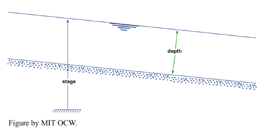
Stage. The stage of a river is the height of the water surface of the stream above an arbitrary datum, usually either sea level or an elevation slightly below the channel bed (Figure 5-1). Stage is related to depth, but the two are not the same.

Figure 5-1. The stage and depth of a river.

The stage of a river is fairly easy to measure. Various kinds of stream gauges are in use. The simplest is a permanent vertical surface with vertical scale markings you read directly on a regular basis. What’s more desirable, but also much more expensive, is an automatically and continuously recording gauge. There are various kinds of such gauges in use; most common is a float gauge, in a stilling well, connected to a strip-chart recorder (Figure 5-2).

Figure 5-2. A stream-gauging station.

Discharge. The discharge of a river is the volume rate of flow past a given cross section, measured in cubic feet per second, cfs (cusecs) or cubic meters per second, m³/s (cumecs). It’s not nearly as easy to measure discharge as it is to measure stage. Most measurement of river discharge makes use of a simple equation that relates discharge Q past a cross section to the area A of the cross section and the mean velocity U of flow past that cross section:

\[Q = UA \label{1}\]

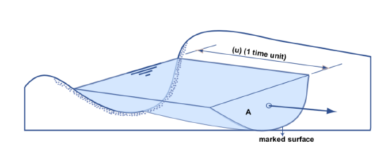
If Equation 1 doesn’t make sense to you immediately, just imagine that at a given instant you could magically mark the water that’s passing through the given cross section and then watch that marked surface drift downstream for a unit interval of time (Figure 5-3). The distance traveled by that surface is, on the average, equal to the mean velocity U, because velocity is distance per unit time. The volume of water between the given cross section and the marked surface after that unit time, which by definition is just the discharge Q, is the product of the cross-sectional area A and the distance traveled by the surface during that unit time, which is equal to the velocity U, times 1, the unit of time.

So if you measure cross-sectional area and mean flow velocity you can solve for the discharge. This is easier said than done, but it’s what’s done in practice. There’s an elaborate set of practical guidelines for doing this in natural streams; the procedure basically involves

• taking a large number of positions across the stream,
• measuring depth-averaged mean velocity (and depth), at each position, and then
• computing and averaging.

Figure 5-3. Seeing what is meant by Equation 1 for river discharge.

Obviously there’s a certain unavoidable sloppiness to this, especially under difficult high-water conditions. It’s done from bridges, cableways, or boats. The accuracy is something like 5% at best, 10–15% at worst. One tries to do it fast relative to change in stage and discharge.

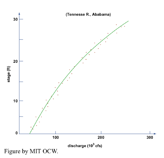
Clearly, you can’t measure the discharge continuously, or even often. But it’s important to be able to know the discharge at times you don’t (or can’t) measure it. How do you derive a continuous record of discharge? The technique involves what is called a stage-discharge diagram, often called a rating curve. The rationale is that if downstream conditions don’t change (for example, by aggradation or degradation occasioned by new structures built upstream, or the shifting of meander bends upstream) this curve is the same all the time, so once you have it you can find the discharge satisfactorily just by knowing the stage and going into the diagram. A lot of effort goes into deriving and checking rating curves. Rating curves are usually convex upward, as in Figure 5-4.

Hydrographs

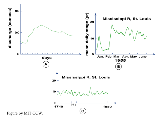
It should seem natural to plot the results of streamflow measurements in the form of a graph of stage vs. time or discharge vs. time. The latter is most common and useful. Both kinds of graph are called hydrographs. Time scales and discharge data used in hydrographs vary widely:

• To study individual floods, you need a “continuous” record of discharge for days or weeks (Figure 5-5A).
• A common longer-term hydrograph shows peak or mean daily discharge for a whole year (Figure 5-5B).
• Longer-term hydrographs show mean monthly or annual discharge over many years (Figure 5-5C). Hydrographs vary widely from river to river depending on climate and substrate. This reflects the circumstance that rivers can be flashy or steady.

Figure 5-4. Example of a rating curve.

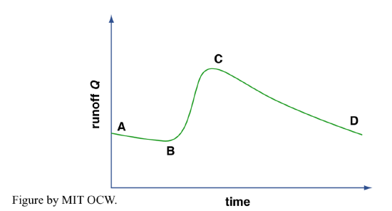
What is the characteristic or typical short-period hydrograph of a stream produced by a rainfall of given duration with given steady intensity? Refer to Figure 5-6.

AB: end of spell without rainfall; all surface runoff has ceased, and groundwater runoff is gradually decreasing.

B: surface runoff from a rainstorm reaches the channel.

BC: this is the rising limb of the hydrograph; surface runoff increases sharply.

C: this is the peak or crest of the hydrograph; surface runoff peaks.

Figure 5-5. Examples of rating curves. A) Discharge hydrograph of n individual flood (conceptual). B) Stage hydrograph of the Mississippi River at St. Louis for an entire year. C) Stage hydrograph of the Mississippi River for over two centuries.

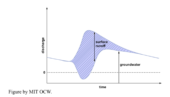
It’s also possible to show both surface runoff and groundwater runoff on the same hydrograph (Figure 5-7). Note that sometimes groundwater flow actually goes negative, because of bank storage: instead of the groundwater feeding the river, the river feeds the groundwater table.

Figure 5-6. Characteristic short-period hydrograph of a stream, associated with a rainfall event of short duration and steady intensity.

Figure 5-7. Showing surface runoff and groundwater runoff on the same hydrograph.

How does one account for the shape of the rising limb of the hydrograph? Think about a tiny “drop” of water falling on the watershed. Assume that it’s not infiltrated or reevaporated but travels as surface runoff. At first it travels as overland flow, and then later as channelized flow. (In fact, watersheds can be classified as “small” or “large” depending on whether the ratio of time involved in overland flow to time involved in channel flow is large or small, respectively.) Eventually the drop passes a given station at the outlet of the drainage basin. This takes a certain average time. You can imagine a map of the drainage basin upstream of this point as being contoured by isochrons (curves of equal travel time) (Figure 5-8)—although it would be very difficult to compute or measure this in actual practice.)

Figure 5-8. Map of a small drainage basin, showing isochrons of equal travel times of surface runoff to the outlet of the basin.

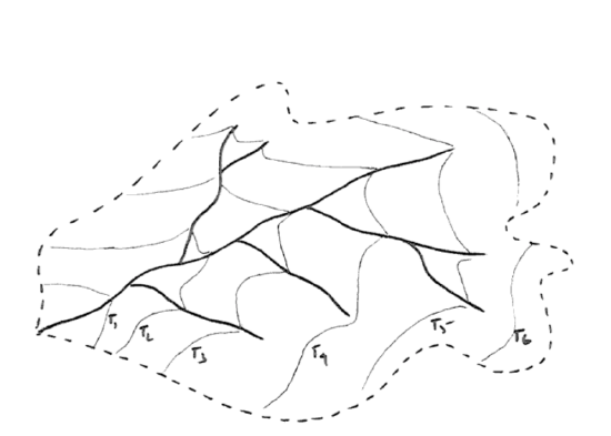
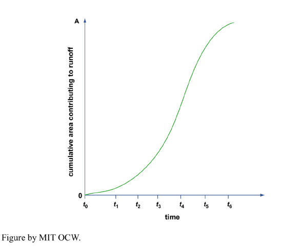
Assume a brief and uniform rainfall over the watershed (that is, the rain doesn’t last long, and the rate of precipitation is the same everywhere in the basin). Surface runoff at our station can be accounted for by looking at cumulative area as a function of time (Figure 5-9). For our brief and uniform storm, this should be equivalent to the rising limb of the hydrograph for this storm if we make the transformation

Runoff = (rainfall depth) times (area)

It should make sense to you that the time it takes to reach the peak of the hydrograph thus derived (that is, the time it takes until all of the watershed area is now contributing to the discharge at the station) gets longer as the watershed area gets bigger. We haven’t dealt with the falling limb of the hydrograph here, but, obviously, after the rain stops, less and less of the watershed area is contributing water, so the discharge past our station gradually decreases.

A hydrograph is this simple only for an ideal rainstorm in a very small watershed. Hydrographs of real rivers are invariably more complicated, for obvious reasons involving unsteadiness (varies with time) and non-uniformity (varies from place to place) of rainfall.

It’s difficult to say anything striking about hydrographs at this point, but the differences in discharge reflected in the hydrographs are of paramount importance in both the channel pattern and the sedimentary processes in streams.

Figure 5-8.

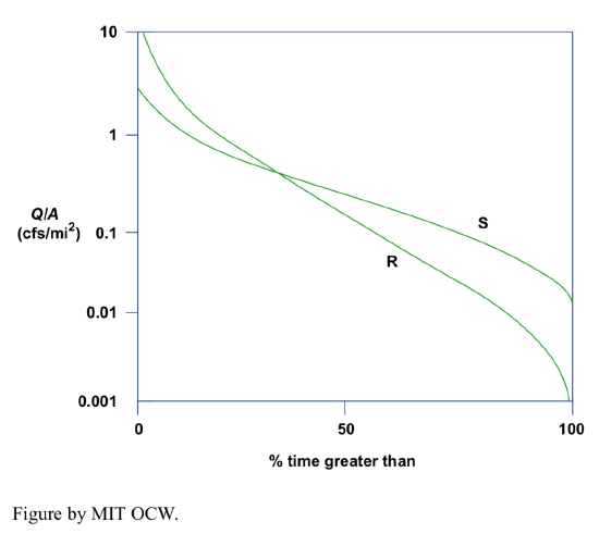
In terms of flashiness (qualitative magnitude of change in discharge from time to time), one of the most important aspects of river behavior for sedimentation, you can plot a similar diagram of discharge vs. percentage of time (this is called a flow-duration curve (or a discharge-duration curve) if you have a long record of discharge. Figure 5-10 shows such a curve for two medium-size streams in Ohio, of about the same size and discharge:

1. Sandy Creek, Sandyville, Ohio: A = 481 mi², underlain by surficial sand and gravel, good porous aquifers;
2. Rocky River, Berea, Ohio, A = 269 mi^₂, glacial till and clay, highly impermeable material.

On the vertical axis is plotted Q/A instead of just Q, to normalize for the area of the drainage basin.

The curve for Rocky River shows greater peak flows and lesser base flows; this is described as flashy behavior. Sandy Creek, on the other hand, shows lesser peak flows and greater base flows; this kind of behavior is steadier and not as flashy.

Figure 5-10. Discharge–duration curve for two small rivers in Ohio.