
1.8: Change detection
- Page ID
- 17279

\( \newcommand{\vecs}[1]{\overset { \scriptstyle \rightharpoonup} {\mathbf{#1}} } \)
\( \newcommand{\vecd}[1]{\overset{-\!-\!\rightharpoonup}{\vphantom{a}\smash {#1}}} \)
\( \newcommand{\dsum}{\displaystyle\sum\limits} \)
\( \newcommand{\dint}{\displaystyle\int\limits} \)
\( \newcommand{\dlim}{\displaystyle\lim\limits} \)
\( \newcommand{\id}{\mathrm{id}}\) \( \newcommand{\Span}{\mathrm{span}}\)
( \newcommand{\kernel}{\mathrm{null}\,}\) \( \newcommand{\range}{\mathrm{range}\,}\)
\( \newcommand{\RealPart}{\mathrm{Re}}\) \( \newcommand{\ImaginaryPart}{\mathrm{Im}}\)
\( \newcommand{\Argument}{\mathrm{Arg}}\) \( \newcommand{\norm}[1]{\| #1 \|}\)
\( \newcommand{\inner}[2]{\langle #1, #2 \rangle}\)
\( \newcommand{\Span}{\mathrm{span}}\)
\( \newcommand{\id}{\mathrm{id}}\)
\( \newcommand{\Span}{\mathrm{span}}\)
\( \newcommand{\kernel}{\mathrm{null}\,}\)
\( \newcommand{\range}{\mathrm{range}\,}\)
\( \newcommand{\RealPart}{\mathrm{Re}}\)
\( \newcommand{\ImaginaryPart}{\mathrm{Im}}\)
\( \newcommand{\Argument}{\mathrm{Arg}}\)
\( \newcommand{\norm}[1]{\| #1 \|}\)
\( \newcommand{\inner}[2]{\langle #1, #2 \rangle}\)
\( \newcommand{\Span}{\mathrm{span}}\) \( \newcommand{\AA}{\unicode[.8,0]{x212B}}\)
\( \newcommand{\vectorA}[1]{\vec{#1}} % arrow\)
\( \newcommand{\vectorAt}[1]{\vec{\text{#1}}} % arrow\)
\( \newcommand{\vectorB}[1]{\overset { \scriptstyle \rightharpoonup} {\mathbf{#1}} } \)
\( \newcommand{\vectorC}[1]{\textbf{#1}} \)
\( \newcommand{\vectorD}[1]{\overrightarrow{#1}} \)
\( \newcommand{\vectorDt}[1]{\overrightarrow{\text{#1}}} \)
\( \newcommand{\vectE}[1]{\overset{-\!-\!\rightharpoonup}{\vphantom{a}\smash{\mathbf {#1}}}} \)
\( \newcommand{\vecs}[1]{\overset { \scriptstyle \rightharpoonup} {\mathbf{#1}} } \)
\(\newcommand{\longvect}{\overrightarrow}\)
\( \newcommand{\vecd}[1]{\overset{-\!-\!\rightharpoonup}{\vphantom{a}\smash {#1}}} \)
\(\newcommand{\avec}{\mathbf a}\) \(\newcommand{\bvec}{\mathbf b}\) \(\newcommand{\cvec}{\mathbf c}\) \(\newcommand{\dvec}{\mathbf d}\) \(\newcommand{\dtil}{\widetilde{\mathbf d}}\) \(\newcommand{\evec}{\mathbf e}\) \(\newcommand{\fvec}{\mathbf f}\) \(\newcommand{\nvec}{\mathbf n}\) \(\newcommand{\pvec}{\mathbf p}\) \(\newcommand{\qvec}{\mathbf q}\) \(\newcommand{\svec}{\mathbf s}\) \(\newcommand{\tvec}{\mathbf t}\) \(\newcommand{\uvec}{\mathbf u}\) \(\newcommand{\vvec}{\mathbf v}\) \(\newcommand{\wvec}{\mathbf w}\) \(\newcommand{\xvec}{\mathbf x}\) \(\newcommand{\yvec}{\mathbf y}\) \(\newcommand{\zvec}{\mathbf z}\) \(\newcommand{\rvec}{\mathbf r}\) \(\newcommand{\mvec}{\mathbf m}\) \(\newcommand{\zerovec}{\mathbf 0}\) \(\newcommand{\onevec}{\mathbf 1}\) \(\newcommand{\real}{\mathbb R}\) \(\newcommand{\twovec}[2]{\left[\begin{array}{r}#1 \\ #2 \end{array}\right]}\) \(\newcommand{\ctwovec}[2]{\left[\begin{array}{c}#1 \\ #2 \end{array}\right]}\) \(\newcommand{\threevec}[3]{\left[\begin{array}{r}#1 \\ #2 \\ #3 \end{array}\right]}\) \(\newcommand{\cthreevec}[3]{\left[\begin{array}{c}#1 \\ #2 \\ #3 \end{array}\right]}\) \(\newcommand{\fourvec}[4]{\left[\begin{array}{r}#1 \\ #2 \\ #3 \\ #4 \end{array}\right]}\) \(\newcommand{\cfourvec}[4]{\left[\begin{array}{c}#1 \\ #2 \\ #3 \\ #4 \end{array}\right]}\) \(\newcommand{\fivevec}[5]{\left[\begin{array}{r}#1 \\ #2 \\ #3 \\ #4 \\ #5 \\ \end{array}\right]}\) \(\newcommand{\cfivevec}[5]{\left[\begin{array}{c}#1 \\ #2 \\ #3 \\ #4 \\ #5 \\ \end{array}\right]}\) \(\newcommand{\mattwo}[4]{\left[\begin{array}{rr}#1 \amp #2 \\ #3 \amp #4 \\ \end{array}\right]}\) \(\newcommand{\laspan}[1]{\text{Span}\{#1\}}\) \(\newcommand{\bcal}{\cal B}\) \(\newcommand{\ccal}{\cal C}\) \(\newcommand{\scal}{\cal S}\) \(\newcommand{\wcal}{\cal W}\) \(\newcommand{\ecal}{\cal E}\) \(\newcommand{\coords}[2]{\left\{#1\right\}_{#2}}\) \(\newcommand{\gray}[1]{\color{gray}{#1}}\) \(\newcommand{\lgray}[1]{\color{lightgray}{#1}}\) \(\newcommand{\rank}{\operatorname{rank}}\) \(\newcommand{\row}{\text{Row}}\) \(\newcommand{\col}{\text{Col}}\) \(\renewcommand{\row}{\text{Row}}\) \(\newcommand{\nul}{\text{Nul}}\) \(\newcommand{\var}{\text{Var}}\) \(\newcommand{\corr}{\text{corr}}\) \(\newcommand{\len}[1]{\left|#1\right|}\) \(\newcommand{\bbar}{\overline{\bvec}}\) \(\newcommand{\bhat}{\widehat{\bvec}}\) \(\newcommand{\bperp}{\bvec^\perp}\) \(\newcommand{\xhat}{\widehat{\xvec}}\) \(\newcommand{\vhat}{\widehat{\vvec}}\) \(\newcommand{\uhat}{\widehat{\uvec}}\) \(\newcommand{\what}{\widehat{\wvec}}\) \(\newcommand{\Sighat}{\widehat{\Sigma}}\) \(\newcommand{\lt}{<}\) \(\newcommand{\gt}{>}\) \(\newcommand{\amp}{&}\) \(\definecolor{fillinmathshade}{gray}{0.9}\)Much environmental change occurs at temporal and spatial scales that make it challenging and potentially costly to study. Obvious examples include some of the manifestations of climate change: the increasing temperatures and melting ice in the Arctic and the subtle vegetation changes occurring throughout Canada, to name a few. Monitoring these things exclusively with field measurements would be incredibly costly, or heavily biased towards populated areas and, when historic measurements are not available, impossible. Remote sensing data come to the rescue here, because aerial photography and satellite imagery is routinely stored and catalogued and they can thus function as data from both the past and the present – as long as we can extract the necessary information from them. Just imagine answering these questions with confidence without having access to remote sensing data:
- Is the annual area burned by forest fires increasing or decreasing in Canada?
- Which part of Canada is warming the fastest?
- Where is there still multi-year ice in the Arctic, and how fast is that area shrinking?
Before we start to use remote sensing data to detect environmental change, it is helpful to consider what we mean by that – what is environmental change? The environment changes all the time – it is snowing outside as I write this and it didn’t snow two days ago – that is a kind of environmental change, but not the kind most people want to detect and map with remote sensing data. Nevertheless, it is exactly that kind of change that is visible in images of the Earth from space, so whether we like it or not we detect a lot of irrelevant change with remote sensing data. To better think about what change we want to detect and what change we don’t, one useful distinction to make is between short-term/instantaneous change and long-term/gradual change. Sometimes we are interested in finding the short-term change, while at other times, when more concerned with longer gradual trends, we consider it noise.
Instantaneous change
Remote sensing can be effective at detecting instantaneous change, i.e. change that happens between one image acquisition and the next. This change may not necessarily be instantaneous in the strict sense of the word, but for practical remote sensing purposes a change that happens in the period between two image acquisitions can be considered ‘instantaneous’. Detecting such change is often done quite easily with visual interpretation of two images, comparing them side by side to easily identify areas of change. An example of this kind of comparison is shown in Figure 63, which shows changes in an urban area in Taiwan between February (left) and December (right) 2002. The vegetation (red areas) has clearly changed in some places, and so has a few of the other areas. Many image processing algorithms have also been developed for this purpose, to automate the process of finding the areas that have changed; we will look at those later in this chapter.
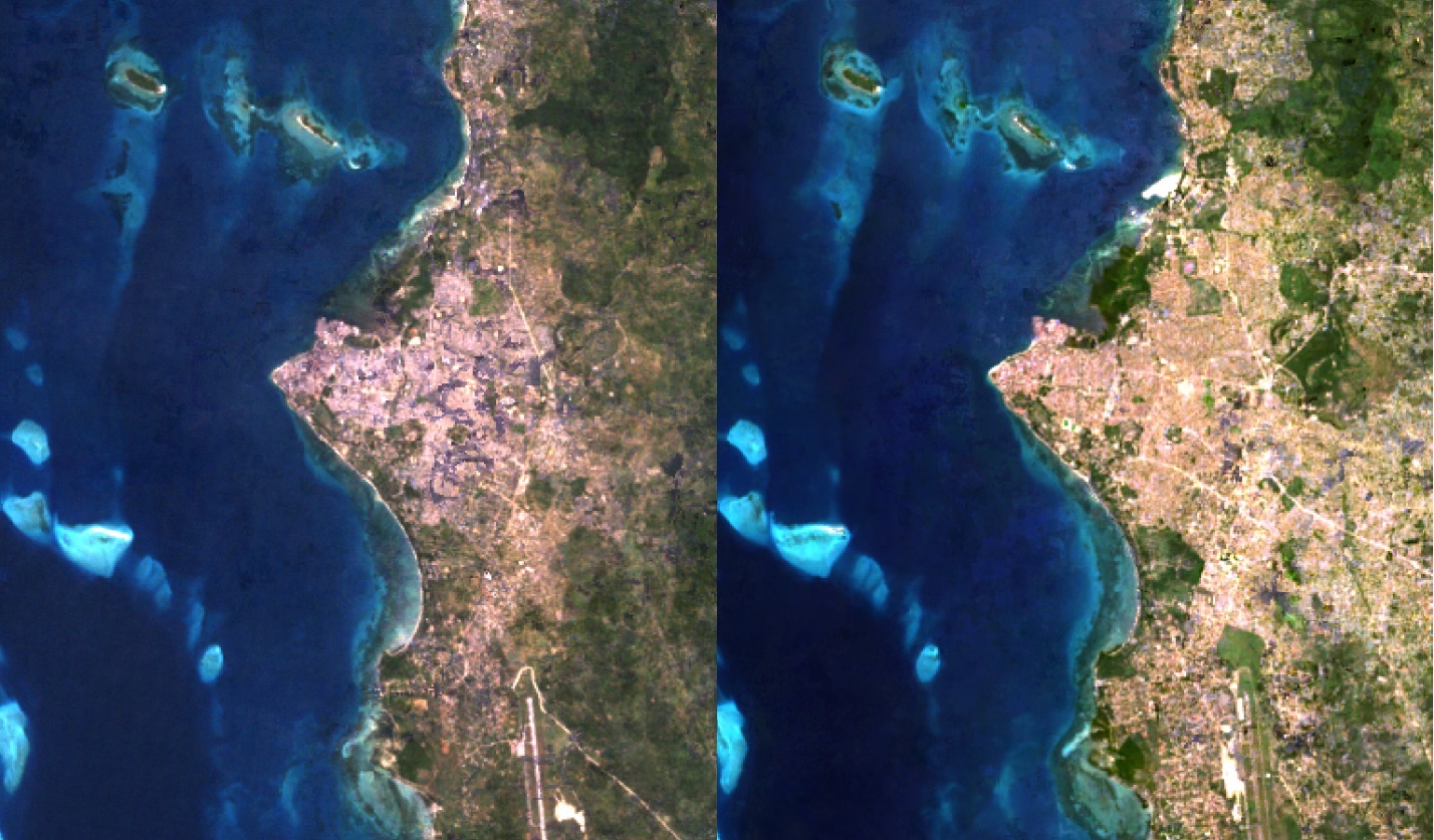
63: Example of side-by-side comparison of two images showing Zanzibar Town in 1995 (left) and 2020 (right). Urban expansion that has occurred in the period between the two images were acquired can be identified visually or algorithmically. By Anders Knudby, CC BY 4.0.
Gradual change
Visual or other image-image comparison can be effective in highlighting obvious abrupt changes such as those caused by urban development, landslides, forest fires and so on. However, more subtle change, such as annual or decadal variation in soil moisture or vegetation health, or change in the depth of the winter snow pack, often requires a different approach to change detection, one that relies on quantitative analysis of changes observed over many images. This is especially the case when individual image-to-image changes may obscure the more gradual long-term trend because of weather-related or seasonal patterns. For example, to study how climate change is affecting vegetation patterns in the Canadian Arctic, a comparison of two images provides, at best, a snapshot of the years those images are from, and at worst it simply tells us that there is more vegetation in 2002 (August) than there was in 1994 (February), which really has nothing to do with a change between the two years but rather is a function of the time of year each image was acquired. Either way, such image-to-image comparisons do not tell us very much about the long-term trend. Instead, a measure of the variable of interest (e.g. vegetation density or health) must be quantified at regular intervals over a long time period to detect such trends. An example is provided in Figure 64, in which the extent of Arctic Sea Ice has been quantified on a near-daily basis for the period 1979 – 2018.
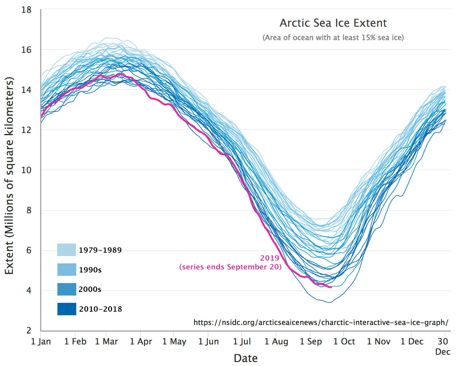
64: Near-daily estimates of Arctic Sea Ice extent. Arctic Sea Ice Extent by M. Scott, National Snow & Ice Data Center (NSIDC), NSIDC Use and Copyright.
The specific methodology used to detect long-term gradual change depends entirely on the kind of change in question (e.g. vegetation vs. sea ice change), so it is difficult to provide details about how to go about detecting change in this case. However, one core concern for any such kind of ‘trend detection’ is that the estimate (e.g. of sea ice extent) should be relatively unbiased throughout the period of observation. In other words, sea ice extent should neither be under- or over-estimated in the 1979-1989 period, and should also neither be under- or over-estimated in 2010s, or at any point in between. This is important to avoid ‘detecting’ trends that are caused by bias in data acquisition or processing, but do not exist in reality.
Separating noise from actual instantaneous change
When comparing one image to another with the intent to detect changes between them, the principal challenge is to detect real environmental change while not detecting change that hasn’t actually happened. As is always the case in binary classification (which this is an example of), there are four possible combinations of reality (change or no change) and estimate (change detected vs. no change detected, Table 14):
Table 14: A binary classification (one that involves two categorical options) can be described with a table like this one. For any image processing system, the challenge in binary classification is to optimize the number/rate of true positives and true negatives.
|
Change detected |
No change detected |
|
|
Change |
True positive (TP) |
False negative (FN) |
|
No change |
False positive (FP) |
True negative (TN) |
The goal, then, is to optimize the rate at which true positives and true negatives are found. Most change detection algorithms operate on a pixel-by-pixel basis, so this means correctly detecting pixels that have actually changed without incorrectly ‘detecting’ change in pixels that have not changed. To do this, we need a way to separate three different situations, each of which can occur in a given pixel:
- No change: the pixel literally looks exactly the same in each image.
- Noise: The pixel looks different in the two images, but the difference is small enough that it is probably caused by factors unrelated to real environmental change. These can include differences in atmospheric conditions between the two images, random noise in the images, imperfect georeferencing, and other issues.
- Actual change: Real environmental change has happened in the pixel, and it shows as a substantial difference between how the pixel looks in the first image and in the second image.
The first situation, no change, happens very rarely because there is noise inherent to the image creation process, and this noise is unlikely to be identical between two different images. The real challenge, then, is to separate situations 2) and 3). There are two principles involved in doing this.
Noise reduction
First of all, it is important to remove as many sources of noise as possible before comparing the data in the two images. Some strategies often employed to this end include:
- Use ‘anniversary dates’. Choose two images that were captured on the same date (or almost) in different years. This is a good way to eliminate large differences between each image related to seasonal changes in soil moisture, vegetation state, snow cover, and other environmental factors that change with the seasons.
- Use images captured by the same sensor. Given that no sensor is perfectly calibrated, using images from two different sensors could potentially introduce a difference that is sensor-based rather than environment-based. For example, if radiance in the 500-600 nm spectrum is slightly overestimated by one sensor and slightly underestimated by another sensor, comparing images between the two may ‘detect change’ where none exists.
- Use images captured at similar atmospheric states. This is difficult because we often don’t have accurate information on aerosol loads, water vapour, wind speed etc., but definitely avoid comparing images with obvious differences in haze, visibility, and other visible atmospheric factors.
- Compare images based on their surface reflectance rather than TOA radiance or TOA reflectance. This is because surface reflectance is a physical attribute of the surface, and is at least in principle independent of atmospheric state and illumination.
- For tilting sensors, if possible compare images taken at more or less the same geometry.
Identifying a threshold
Once as many sources of noise as possible have been eliminated, and the images have been converted to surface reflectance for comparison, there will still be some noise that causes surface reflectance values in the two images to differ slightly between the images, even for pixels that have not experienced the kind of change we want to detect. To separate situations 2) and 3) above, it is therefore important to consider what ‘real’ environmental change means and define a threshold below which any ‘change’ observed in the image comparison is considered ‘noise’ rather than ‘real change’. For example, imagine that you are studying changes in vegetation, and you have two images of the same forest. The real change that happened between these two images is that one leaf fell off one of the trees in the forest. This is an actual observable change in the environment, but in any real sense it does not warrant the label ‘deforestation’! One prerequisite for separating situations 2) and 3) above then is to define how much change is required for you to consider the area ‘changed’. Unless you have field observations (and you typically don’t because change is detected backwards in time and you cannot go and get field data from the past), this requires defining the threshold based on the images themselves, something that is typically an interactive and subjective process.
Methods for detecting instantaneous change
Some of the simplest approaches to detecting the magnitude of change are based on ‘image math’.
Band difference
For example, the magnitude of change can be defined as the difference between surface reflectance values in band 1 in the two images, plus the difference in band 2, etc.:
Band ratio
Or ratios can be used instead of differences:
Euclidian distance
A more commonly used method is to calculate the ‘Euclidian Distance’, using each band as a dimension and each image as a point. Imagine that you plot the surface reflectances of each image as points in a coordinate system. The Euclidian distance between them would then equal:
For each of these approaches, to separate noise from real environmental change, a threshold value will need to be defined. Pixels that have experienced no change or change smaller than the threshold value will then be considered effectively ‘unchanged’, while those that have experienced more change will be considered to contain ‘real change’. Also note that for each of these approaches, the number of bands involved in the calculation have been limited to two in the equations above, but can be extended to include any number of bands present in the images.
Methods for detecting and attributing instantaneous change
All three above approaches can be effective at detecting change, but they also all suffer from the drawback that they tell us very little about the kind of change that has happened in a given pixel. While detection of change is a great first step, it is not easy to base management decisions on, so figuring out a bit more about the kind of change that has been detected, called change attribution, is useful.
Change vectors
Change vectors can help with this. Change vector analysis is an extension of calculating the Euclidian distance, in which the direction of change is also calculated. An example with only two dimensions is provided in Figure 65. In the ‘before’ image, the surface reflectance value in band 1 is 0.1, and the NDVI value is 0.5. In the ‘after’ image, these values have changed to 0.3 and -0.2 respectively. This illustrates two things: 1) you do not need to use actual band values as inputs to change detection analyses, and 2) the direction of change – increase in band 1 reflectance, decrease in NDVI, can be found.
In change vector analysis, the magnitude of change is calculated as the Euclidian distance, as per the equation above. The direction of change can be calculated in degrees (e.g. compass direction) or, to ease interpretability, in major directions: A) up and right, B) down and right, C) down and left, D) up and left. If the ‘bands’ used can be interpreted in a meaningful way, attributing the change can be easy. Changes that involve a decrease in a vegetation index involve a loss of vegetation, while those that lead to an increase in, say, surface temperature involve, well, an increase in surface temperature (these two often go together because vegetation helps keep a surface cool). While calculating Euclidian distance is easy when more than two dimensions are used in change vector analysis – you just extend the equation to contain more terms – the direction of change becomes more difficult to define and categories are typically developed for a specific application. As with the methods simply used to detect change, a threshold can be applied to the magnitude of the change vector, below which ‘no change’ is detected.
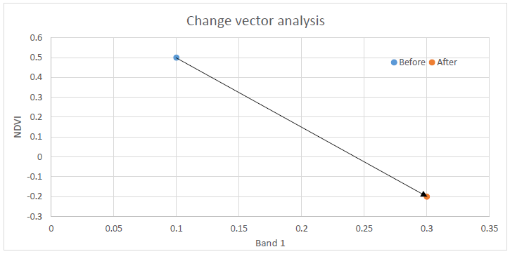
65: Example of change vector analysis with only two bands. NDVI is the Normalized Difference Vegetation Index, described in more detail in the next chapter. Anders Knudby, CC BY 4.0.
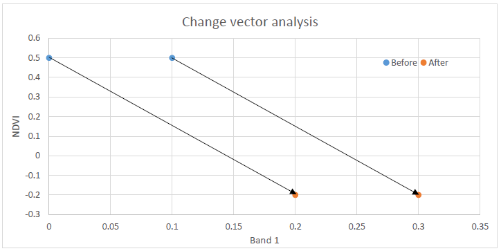
66: One drawback of change vector analysis is that two identical change vectors can represent different kinds of change. Anders Knudby, CC BY 4.0.
One drawback of change vector analysis is that two different changes can have the exact same change vector. For an example, look at the two arrows in Figure 66. While the two vectors are identical – they have the same direction and magnitude – they are likely to represent different kinds of change because they start and end in different places. It is thus difficult, in practice often impossible, to use change vector analysis to specifically figure out what the surface was before and after the change.
Post-classification change detection
Probably the simplest way to both detect and attribute change in an area is to conduct a land cover classification on the ‘before’ image, conduct another land cover classification on the ‘after’ image, and then find pixels that got classified differently in the two images. While this is appealingly straight-forward, and can work occasionally, it is subject to a significant drawback: It is very difficult to produce accurate results in this way. The reason is that no classification is perfect, and when comparing two imperfect classifications the errors combine. I therefore strongly suggest avoiding this approach.
Change classification
If you really want to know what the changed area was before and after the change, an alternative to post-classification change detection is to combine all bands from the two images into a single image. For example, if you have two images, each with six bands, you could ‘stack’ them to get a single 12-band image. This allows you to run a single classification on the 12-band image. With good field data to calibrate this classification each class can be defined according to the combination of before-and-after land covers. The classification can be either supervised or un-supervised, pixel-based or segment-based. This approach allows the two vectors in Figure 66 to end up in two different classes, where maybe one is a change from coniferous forest to marsh while the other is a change from deciduous forest to bog.
Change classification also allows you to remove class combinations that are impossible or highly unlikely, such as a change from ‘ocean’ to ‘coniferous forest’, or from ‘industry’ to ‘wetland’. Deciding which before-after combinations of classes are likely and which are unlikely in a given area requires some expertise, and complex change detection systems are often built using a combination of change vector analysis, change classification, and such expert input.