6.9: Distribution of Surface Sediments

Surface sediments are the materials currently accumulating on top of older sediment. The older sediment buried below the surface layer may have a different character if the deeper layer was deposited under different conditions.

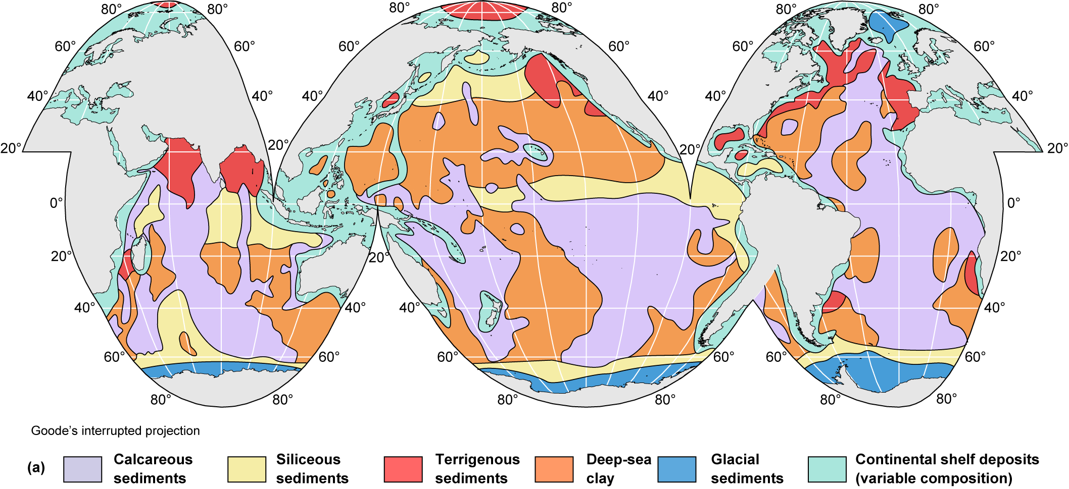
The distribution of pelagic surface sediments and their current rate of accumulation are shown in Figure 6-19. Continental margin sediments are not shown because they are lithogenous except in areas dominated by coral reefs and in some areas of calcium carbonate precipitation. Each type of sediment and the factors that govern its occurrence are described briefly in the sections that follow.

Figure 6-19. Present-day sedimentation. (a) The distribution of present-day surface sediments of the world oceans. (b) Approximate sedimentation rates in the present-day oceans. Note the higher rates of sedimentation near the continents. Surface sediments in these areas are predominantly terrigenous. Sediments are predominantly red clays in areas where the sedimentation rate is lowest. Note the generally slower rate of sediment accumulation on the abyssal floor of the Pacific Ocean compared to that of the Atlantic Ocean.

Radiolarian Oozes

In the Pacific and Indian Oceans, under a region of high productivity that extends in a band across the deep oceans at the equator (Chap. 13), surface sediments are fine muds that consist primarily of radiolarian shells. Although both calcareous and siliceous organisms grow in abundance in this upwelling region, calcareous material dissolves and does not accumulate in sediments below the CCD. Radiolaria (Fig. 6-9) are prolific in tropical waters, and the rate of input of radiolarian shells to the sediment is much higher there than in other deep-sea mud areas. Because siliceous material dissolves slowly, many radiolarian shells are buried in the surface sediment before they fully dissolve.

The rate of input of fine-grained lithogenous particles that are resistant to dissolution is approximately the same in the equatorial band and in the adjacent areas where deep-sea mud accumulates. However, the rate of accumulation of radiolarian shells, and therefore the overall sedimentation rate, is much higher in the equatorial band. Therefore, the deep-sea lithogenous mud particles are “diluted” to become a minor component in radiolarian oozes.

The Atlantic Ocean has no band of radiolarian ooze because the accumulation rate of lithogenous sediment is much higher there than in the tropical Pacific and Indian Oceans, primarily due to the relatively shallow seafloor and the relatively deep CCD. The radiolarian content of tropical Atlantic sediments is diluted and masked by the greater contributions of calcareous and lithogenous sediment. Hence, the overall sedimentation rate in the tropical Atlantic Ocean exceeds the sedimentation rate in the tropical Pacific and Indian oceans.

Diatom Oozes 

Diatoms dominate the siliceous phytoplankton in upwelling areas except in the tropical upwelling zone, where radiolaria dominate. Upwelling and abundant diatom growth occur in a broad band around Antarctica and in the coastal oceans along the west coasts of continents (eastern ocean margins) in subtropical latitudes (Chaps. 8, 13). Diatom oozes dominate in these locations if the sedimentation rates of lithogenous and calcareous particles are relatively slow.

Aside from large coastal inputs from Antarctica’s glaciers, sedimentation in the Southern Ocean is limited because of the lack of landmasses and river inflows. Hence, the accumulation rate of lithogenous particles is slow in the band of high diatom productivity that surrounds Antarctica, and the sediments are dominated by diatom frustules.

Terrigenous sediment inputs are also limited on the west coasts of North and South America because of the limited drainage areas of coastal rivers and the trapping of terrigenous sediment in the trenches that parallel these coasts. Because the seafloor is deep in the Pacific coast upwelling regions and the CCD is relatively shallow in the Pacific Ocean, calcareous particles are dissolved and do not accumulate in sediments. Diatom frustules therefore dominate the sediments in the north and south subtropical Pacific offshore basins. In contrast, on the eastern ocean boundaries in the Atlantic Ocean (southern Europe and West Africa) and Indian Ocean (Australia), in areas where the seafloor is relatively shallow, calcareous particles accumulate faster than diatomaceous particles, and the sediments are calcareous.

Diatoms are very abundant in Northern Hemisphere cold-water regions (Bering Sea and North Atlantic), just as they are near Antarctica. However, lithogenous sediment inputs are greater in the Northern Hemisphere than in the Southern Ocean, and much of the seafloor is above the CCD. Therefore, diatomaceous particles are diluted by calcareous and lithogenous particles, and diatomaceous oozes accumulate only in limited deep areas of the Bering Sea and northwestern Pacific Ocean.

Calcareous Sediments

In areas where the seafloor is shallower than the CCD, calcareous sediment particles accumulate faster than deep-sea clays. Therefore, where the seafloor is shallower than the CCD and terrigenous inputs are limited, calcareous particles are a major component of the sediment. Calcareous sediments are present on oceanic plateaus and seamounts and on the flanks of oceanic ridges.

Deep-Sea Clays

Few large particles are transported into the deep oceans remote from land unless they are carried by turbidity currents (mostly in the Atlantic Ocean). Most deep-ocean areas far from land sustain relatively poor productivity of marine life (Chap. 13). Because of the great depth, the relatively small quantities of biogenous material that fall toward the seafloor are mostly dissolved before reaching, or being buried in, the sediment. This is especially true for calcareous organisms in areas where the seafloor is below the CCD. Therefore, the particles deposited on the deep-sea floor far from land are mainly fine lithogenous quartz grains and clay minerals.

Deep-sea clays (sometimes called “red clays”) are reddish or brownish sediments that consist predominantly of very fine-grained lithogenous material. Everywhere but at high latitudes and in a high productivity band extending across the equatorial Pacific and Indian Oceans, they cover the deep-ocean floor that is remote from land. The reddish or brownish color is due to oxidation of iron to form red iron oxide, which we know as rust, during the slow descent of the particles to the seafloor. Oxidation continues on the seafloor until the particles are buried several millimeters deep. The sedimentation rate is very low, so burial is very slow, and the interval during which oxidation occurs is very long.

Siliceous Red Clay Sediments

In the deep basins of the North and South Pacific, South Atlantic, and southern Indian Oceans, transitional areas are present between the central deep basin, whose surface sediments are red clays, and higher latitudes, where surface sediments are diatom oozes. Sediments in these transitional areas are mixtures of deep-sea clay and diatomaceous sediments in varying proportions. The transitional sediments are often classified with deep-sea clays and often called “deep-sea muds.”

Ice-Rafted Sediments

In the Arctic Ocean, northern Bering Sea, and a band immediately surrounding Antarctica, the sediment consists largely of lithogenous material carried to the oceans by glaciers. It includes sand, pebbles, and even boulders up to several hundred kilometers offshore from the glaciers. Some lithogenous material is released directly to the ocean when the edge of the ice shelf or glacier melts. Some is transported by icebergs, also called “ice rafts,” that break off the glaciers. The material released and deposited as the ice melts is known as glacial, or “ice-rafted,” debris. Because glaciers can carry huge quantities of eroded rock, the sedimentation rate can be very high. Biogenous particles therefore, are diluted by and mixed with much larger volumes of ice-rafted lithogenous material.

Terrigenous Sediments

Sediments dominated by terrigenous particles are present near the mouths of major rivers and may extend hundreds of kilometers offshore. Such sediments are deposited in the northern Arabian Sea, the Bay of Bengal, the Gulf of Mexico, and the Atlantic Ocean near the mouth of the Amazon River in Brazil. Terrigenous sediments transported by turbidity currents are present at the foot of the continental slope in the North Atlantic. On the North Pacific coast of North America, rivers carry large sediment loads from the glaciers in the mountains of British Columbia and Alaska. Many of the glaciers terminate and melt before reaching the ocean. Ice rafts are few, so coarse sand, pebbles, and boulders are not transported beyond the immediate vicinity of the glacier termination. However, large quantities of glacially ground sand, silt, and mud are transported to the ocean by rivers, and offshore by waves and currents.

Hydrothermal Sediments

The central basin of the Red Sea is the only area known to have hydrothermal mineral deposits as the dominant sediment type. The other locations where such sediments accumulate are small and scattered throughout the oceans, mostly on the oceanic ridges. The extent of such deposits is not known because only a very tiny fraction of the oceanic ridge system has been surveyed by methods that reveal hydrothermal vents and their associated sediments. Vents have been found on oceanic ridges in all oceans and are likely to be present at intervals of a few kilometers to hundreds of kilometers along the entire oceanic ridge system.