3.3: Plate Boundaries and Interiors

Transform Boundaries

Figure \(\PageIndex{1}\): The modern plate boundary in the San Francisco region formed as the plates slide past one another, seen here south of San Francisco along the trace of the San Andreas Fault. (Callan Bentley photo.)

Transform boundaries are the simplest kind of plate boundary. At a transform boundary, new lithosphere is neither created nor destroyed. Instead, the two plates slide past one another in opposite directions. Friction acts to restrain the plates’ motion. Moments when the friction is overcome — and the plates slip rapidly and violently — are earthquakes. Earthquakes are the main geological phenomenon to be aware of at transform boundaries, but the earthquakes there are distinct in that they are relatively shallow (20 km deep or less), and range in magnitude between small and large (~M7.5 at the most), but they are never huge, like the largest quakes that can occur (~M9) at convergent boundaries. This difference in magnitude occurs as rock is weaker under shear stress (stress generated when materials try to slide past one another) than under compressional stress (stress generated when materials are pushed together), so less stress builds up at transform boundaries.

Transform boundaries can be recognized by offset features that cross the plate boundary such as bodies of rock, landscape features such as stream valleys, or human-built structures such as roads and fences.

Watch this 50-second video as a geologist shows where the San Andreas Fault offset a stream. You can see the offset where the stream cuts to the right in the video.

Figure \(\PageIndex{2}\): Crushing of bedrock on the San Andreas Fault in California has encouraged differential erosion of the landscape, producing the Olema Valley and Tomales Bay. (Landsat image from NASA.)

As a result of the stress and subsequent breakage of rock along the boundary, fault zones are created. Because crushed-up, pulverized rock weathers and erodes more rapidly than unbroken rock, the landscape of transform boundaries frequently shows linear features parallel to the trace of the fault zone: straight valleys and coastlines, elongated peninsulas, and bays.

In places where the trace of the faults on a transform boundary bend, the fault is no longer parallel to the plates’ motion. This results in localized areas of compression (pushing forces) or tension (pulling forces). When compression results, rock is forced upward into a pressure ridge. Pressure ridges can be small enough to see in a parking lot pavement, or the size of mountains. When tension results, land drops down. If it is a small feature and it fills with water it is called a sag pond. If it is a bigger feature and fills with water, it can make a larger trough like the Salton Sea.

Figure \(\PageIndex{3}\): A small pressure ridge developed in parking lot asphalt at Central Park, Fremont, California. The plate motions are indicated by the large arrows. The bend in the fault and subsequent compression is indicated with the smaller arrows. Perspective is looking to the southwest across the fault. (Callan Bentley photo.)

Figure \(\PageIndex{4}\): A sag pond developed along the North Anatolian Fault in Turkey. (Callan Bentley photo.)

Continental transform boundaries are striking, but far more common are examples of transform faults in the oceanic lithosphere. Between segments of oceanic ridge on the seafloor are zones where the plates slide past one another. These are oceanic transform faults, and they are a key feature of overall divergent boundaries in our planet’s ocean basins. Together with the oceanic ridges you’ll learn about below, the create the distinctive zigzag shape to most oceanic divergent plate boundaries.

Figure \(\PageIndex{5}\): The oceanic ridge system comes in many segments, offset along perpendicular fracture sets. The big arrows show the divergence at the plate boundary. The smaller red arrows show where slipping is occurring along transform boundaries.

Divergent Boundaries

Divergent boundaries are sites where two plates move away from one another. In this extensional setting the crust thins while it stretches out laterally. Divergent boundaries come in two principal varieties that are relevant to geology:

• rift valleys in continental crust
• oceanic ridges in oceanic crust

Rift Valleys in Continental Crust

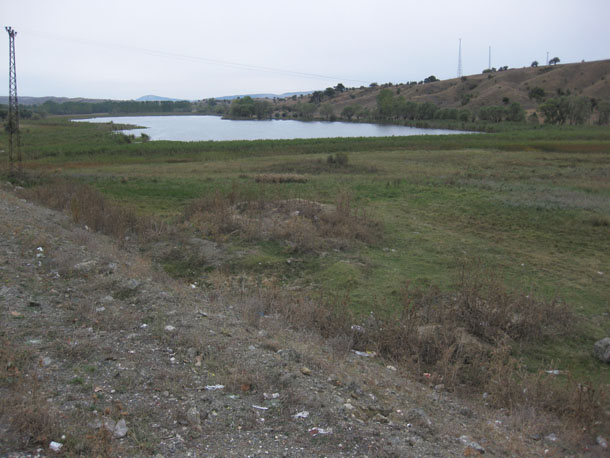
When a divergent boundary develops in continental crust, blocks of crust drop down into the gap created producing an elongated low spot called a rift valley. The classic modern example is the Great Rift Valley of east Africa (pictured here).

Figure \(\PageIndex{6}\): A fresh divergent boundary developing in continental lithosphere, east Africa. (NASA photo, annotated by Callan Bentley.)

The edges of the rift valley are high in elevation, which encourages sediment (loose material) to drop from the surrounding highlands into the rift valley. This sediment does not travel far, or for very long so material of various sizes and compositions pile up along these rift valley edges, smoothing out the highest relief areas. Smaller sediment gets carried a bit further, and creates deposits of sand. Water accumulate in the lowest regions, furthest from the rift valley edge, forming lakes that grow salty as they evaporate.

A very similar distribution of rocks and sediment can be seen in older, now-inactive rift valleys. For instance, the Culpeper Basin of central Virginia was an active site of rifting during the Triassic and Jurassic periods (150-250 million years ago), as the supercontinent Pangaea was breaking apart and the Atlantic Ocean was first forming.

Crustal thinning also allows molten material to rise to the surface. As the plates move apart at the divergent boundary, mantle material rises up. As the pressure is reduced, melting occurs without the addition of any new heat. This molten material may rise to the surface to erupt as “floods” of liquidy lava. This is seen as a large black patches in the satellite image above, showing the Afar Triangle region of northeastern Africa.

Figure \(\PageIndex{7}\): Volcanic ash from rift valley volcanism preserves trace fossils of hominids that walked upright.

As the rising molten material interacts with the crust on its ascent, it can transfer some of its heat and produce larger bodies of molten material, resulting in large volcanoes such as Mt. Kenya, Mt. Kilimanjaro, or Mt. Meru. It was ash erupted at one of these large volcanoes in the East African Rift Valley that preserved the footprints of two Australopithecines waking side by side at Laetoli, Tanzania, 3.2 million years ago.

Continental rifting is only the beginning of a divergent boundary however. Once the crust is sufficiently thinned, a process called seafloor spreading takes over. This can be seen just north of East Africa, where a narrow body of oceanic crust separates Africa from Arabia. These gaps are filled with water creating the Red Sea and the Gulf of Aden. They are just a bit more ‘tectonically mature’ than the Great Rift Valley, which is not thinned enough to allow ocean water to flood it creating a sea.

Figure \(\PageIndex{8}\): Junction of the African (Nubian), African (Somalian), and Arabian plates showing how the East African Rift has not dropped low enough for water to flood it like what has occurred to form the Red Sea and Gulf of Aden. Used under the CC BY 3.0 license.

Here, the continental crust has fully broken into two discrete separate segments, diverging as Arabia moves to the northeast. New oceanic crust is filling the gap between them, a process called seafloor spreading.

Oceanic Ridges in Oceanic Crust

When oceanic lithosphere diverges and seafloor spreading occurs, mantle rises up and the pressure lowers triggering the formation of melt, a process called decompression melting. This melt cools at various depths to produce new oceanic crust. When freshly formed, this oceanic crust makes a high feature on the seafloor, an oceanic ridge (also called a “mid-ocean ridge,” since many of them are in the middle of the ocean basins).

Figure \(\PageIndex{9}\): The formation of sea floor at an oceanic ridge. (USGS, Public Domain)

As the plates continue to diverge, this melt squirts into the cracks. Some of the melt may make it all the way into the water and the bottom of the ocean, erupting to produce pillow basalts (see figure below), while some magma cools rapidly and solidifies in the feeder crack itself, making a what is called a dike (see figure below).

Figure \(\PageIndex{10}\): The formation of pillow structures occurs when melt erupts underwater. (Callan Bentley cartoon.)

This all produces a rock called basalt, which is explained elsewhere in this text. Still more melt cools slowly, deeper in the new oceanic crust, producing bodies of a rock called gabbro which is also explained elsewhere in the text. This sequence of rock types is an ophiolite sequence, an important feature discussed below in the convergent boundaries section.

Seafloor spreading happens at different rates in different ocean basins. The East Pacific Rise in the Pacific Ocean generates roughly twice as much new seafloor in a given amount of time as the Mid-Atlantic Ridge in the Atlantic Ocean. This is seen in the diagram below as young seafloor indicated using red, orange, and yellow covers much more of the Pacific Ocean than the Atlantic.

Figure \(\PageIndex{11}\): Age of the oceanic crust on Earth. (NOAA map.)

Oceanic crust also records the changes in Earth's magnetic field over time, as magnetic north (currently roughly lined up with the Earth's North Pole) flip flops back and forth at irregularly scheduled intervals. The melt that cools to make oceanic crust contains minerals such as magnetite, which will rotate into alignment with Earth’s magnetic field before the melt around them solidifies. The generation of new oceanic crust through seafloor spreading therefore records changes in the polarity of Earth’s magnetic field at any given time and creates a continuous record.

Figure \(\PageIndex{12}\): Spreading along several mid-ocean ridges, showing magnetic striping symmetry. (Animation by Tanya Atwater, UCSB.)

Convergent Boundaries

Convergent boundaries are sites where two plates move toward one another. Depending on whether the leading edge of these two plates consists of oceanic lithosphere or continental lithosphere, several different situations can result.

Oceanic-Continental Convergence

Figure \(\PageIndex{13}\): Key features in an oceanic-continental subduction zone. (Public domain via USGS.)

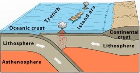
When oceanic lithosphere converges with a continent, subduction happens. Subduction is when the plate of oceanic lithosphere descends down into the mantle beneath the plate of continental lithosphere. This subduction is marked by many phenomena: an oceanic trench (see figure above) marks the place where subduction begins, but earthquakes are generated all along the subduction zone to great depths beneath the overriding plate. The earthquakes at this boundary type can be among the largest known. At the trench, any sediment or other features atop the plate may be scraped off, building up in a thick jumbled pile called an accretionary wedge.

Figure \(\PageIndex{14}\): Osorno (left) and Calbuco (right) are classic Andean volcanoes in Chile marking a oceanic-continental convergent boundary. (Callan Bentley photo.)

As it descends, the subducted plate releases water into the surrounding mantle. This water enables the melting of the mantle rock, generating magma. This magma rises and pools beneath the base of the continental crust, transferring its heat. The minerals of the continental crust tend to have lower melting temperatures, and so they melt, resulting in the creation of a mixed melt, which continues to ascend through the crust. They may lodge at depth, crystallizing to make solid rock bodies called plutons (smaller) and batholiths (bigger), or they may find their way to the surface, where they erupt as volcanoes. The development of a continental volcanic arc (chain of volcanic mountains found along a coastline) parallel to the trench is a sure indication of oceanic-continental convergence.

Several places in the modern world are examples of this kind of plate boundary, including the Cascadia volcanic arc in the Pacific Northwest of the United States of America, but the classic example is the western edge of South America (continental lithosphere), where subduction of the Nazca Plate (oceanic lithosphere) has resulted in the Andes volcanic arc as well as some of the largest earthquakes ever recorded.

Figure \(\PageIndex{14}\): Osorno (left) and Calbuco (right) are classic Andean volcanoes in Chile marking a oceanic-continental convergent boundary. (Callan Bentley photo.)

Figure \(\PageIndex{15}\): Shaded relief map of Earth showing concentration of earthquakes (black dots) and volcanoes (red dots) along plate boundaries which are often along coastlines. (Simkin, et al. (2006), USGS.)

Ancient subduction zone complexes can be found in in many places that are no longer experiencing subduction: coastal California, central Turkey, western France, and the Cyclades of Greece are a few examples. When geologists find these complexes they know subduction occurred there sometime in the past at a convergent boundary.

Oceanic-Oceanic Convergence

Figure \(\PageIndex{16}\): Key features in an oceanic-oceanic subduction zone. (Public domain via USGS.)

When two plates of oceanic lithosphere converge, subduction results when one of the two plates descends beneath the other. Because they are both composed of the same plate type, the key variable is density based on age. Older oceanic lithosphere is colder oceanic lithosphere, and colder rock tends to be denser. For instance, in the western Pacific Ocean, ~200 Ma oceanic lithosphere of the Pacific Plate is subducting beneath ~20 Ma oceanic lithosphere of the Philippine Plate. In a match-up between old and young oceanic lithosphere, the young wins, and the old subducts. Because convergence with both continental lithosphere and young oceanic lithosphere “selects against” old oceanic lithosphere, there is very little of it still around. The oldest oceanic lithosphere left on this planet is Permian in age (~250 Ma), in the Mediterranean Sea.

When old oceanic lithosphere subducts, a trench (see figure above) and an accretionary wedge results, just like when subduction occurs under continental lithosphere. Again the rock of the subducted slab releasing water into the mantle which triggers melting of the mantle. The melt rises up to pierce through the overlying crust as a chain of volcanic islands. We call this a volcanic island arc.

In this overlay of the “Discovering Plate Boundaries” volcanology and topography maps, you can see this relationship plainly: in each location where we see a deep sea trench, it is paralleled by a volcanic island arc (line of red dots):

Figure \(\PageIndex{17}\): There is a strong coincidence of deep sea trenches and parallel belts of volcanoes. (Dale Sawyer’s “Discovering Plate Boundaries” maps.)

Continental-Continental Convergence

Figure \(\PageIndex{18}\): Key features in an continent-continent convergent boundary. (Public domain via USGS.)

The final circumstance that can happen at a convergent plate boundary is when all the oceanic lithosphere separating two continents has been subducted, and the two continents (formerly separated by an ocean basin) finally meet. Because of their buoyancy, the continents cannot subduct very far. Instead, they crumple upward into mountains. Deep below the plate boundary, the plate crumples too, thickening into a root that extends downward. Extending all the way through the thickest lithosphere on the planet, this is a young collisional mountain belt. The act of forming a mountain belt is an orogeny (from the ancient Greek for “mountain making”).

The classic modern example of a collisional mountain belt is the Himalaya, which have been forming for the past ~40 million years where the Indo-Australian Plate is converging with the Eurasian Plate. Frequent large, shallow earthquakes mark this collisional zone, but there is no volcanism since melt is not produced in this process.

Figure \(\PageIndex{19}\): Aerial view over the raw mountains formed as India and Asia collide. (Photograph by Susan Hough; reproduced with permission.)

If the compressional stresses are strong, rocks on the flanks of the mountain belt will be deformed through folding (bending) and faulting (breaking). This zone of compressional deformation is distinct and pervasive in mountain belts across time and space. Examples include the Pyrenees in Spain and France, the Cape Fold Belt in South Africa, the Valley & Ridge province of the Appalachians, the Ouachita Mountains in Arkansas, the Marathon Mountains in Texas, the Caledonides in Scandinavia, the Sevier Fold and Thrust Belt in the Rocky Mountains, the Damara Belt in Namibia, the Atlas and Anti-Atlas in Morocco, and the Alps in Europe.

Figure \(\PageIndex{20}\): Zerrissene turbidites, folded by the Damara Orogeny, Namibia. (Photograph by Jay Kaufman; reproduced with permission.)

Here are a few images highlighting folds created in this way around the world:

Figure \(\PageIndex{21}\): Folded sedimentary layers are a signature of compressional forces associated with mountain-building.

Figure \(\PageIndex{22}\): Google Earth Image of the Appalachian Mountain fold belt in western Pennsylvania at 200 km eye altitude.

Figure \(\PageIndex{23}\): Cape Liptrap (southeast of Melbourne in Victoria, Australia). (Photo by Sandra McLaren.)

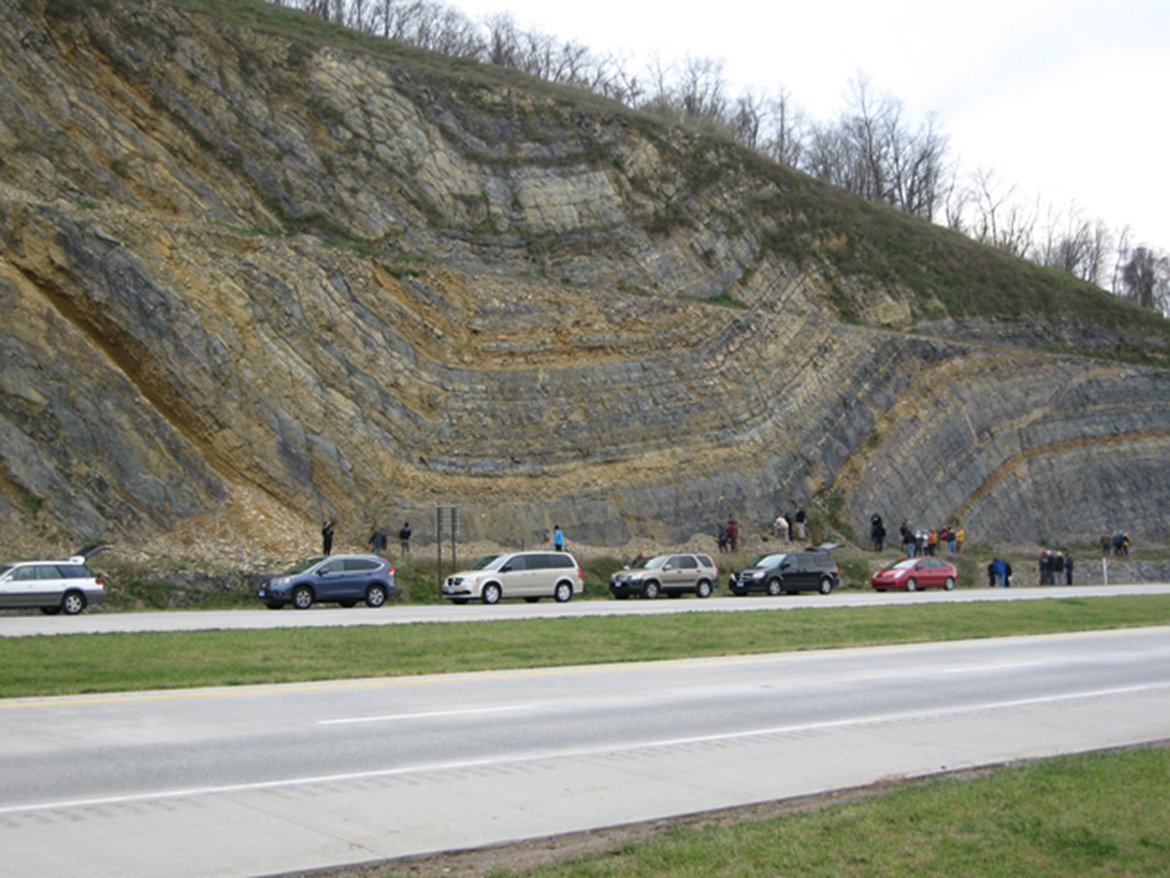
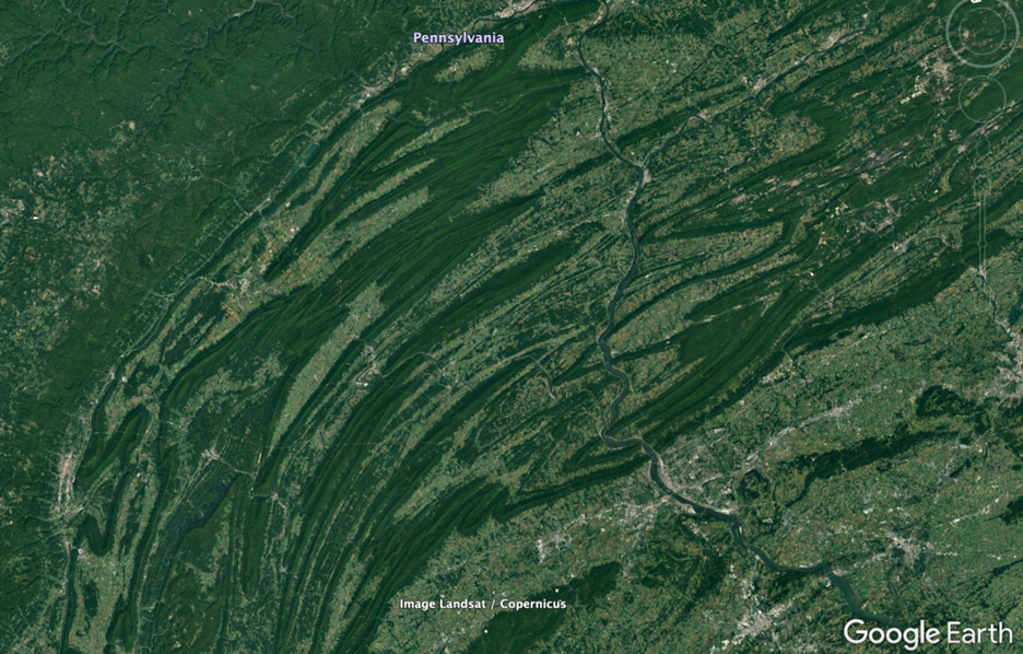
Plate Interiors

Figure \(\PageIndex{24}\): Assateague Beach, Virginia. Note the extremely subdued topography and sand (accumulating mature sediment). (Photo by Doug Kerr via Wikimedia.)

Though most of the geological “action” happens at plate boundaries (edges), the vast interiors of plates merit some attention, too. Largely they move as a single block, traveling in a common direction or rotating around some axis of motion. Passive margins are the “trailing” edges of continents within a plate such that they are marked by coastlines without a plate boundary. For instance, consider the North American continent as it is today. As it moves from east toward the west, the western edge is the active margin where the coastline does mark the plate boundary (with Cascadia subduction and two giant transform fault zones). The eastern edge is the passive margin, trailing along with no active tectonics. A place like Virginia is the edge of the continent, but the middle of the plate. No mountains are being actively built in modern Virginia, but old mountains are being eroded away. Particles of sand and mud with origins in the Appalachian Mountains are tumbled downstream and deposited along the western edge of the the Atlantic Ocean.

A passive margin is a site of tectonic calm. Without plate tectonics to rough up the landscape, the topographic relief is minimal. Cool crust is denser, and subsides. This allows the accumulation of deposits of mature sediment. These sediments have been laid down along the modern mid-Atlantic margin in the thick layers of the Coastal Plain and continental shelf.

Other modern examples of passive margins include eastern South America, Western Africa, Western Australia, and southern India, as plate boundaries do not exist at these coastlines.

Key Terms

• accretionary wedge - structure near an oceanic trench formed by the accumulation of sediment scraped off the subducting oceanic lithosphere and shoved onto the overriding oceanic or continental plate
• active margin - a continental coastline that is marked by a plate boundary
• continental volcanic arc - a chain of volcanoes formed on a continental plate as a result of the subduction of oceanic lithosphere
• convergent boundary - plate boundary type at which the two plates move toward one another
• decompression melting - melting of rock triggered as rock rises and pressure is lowered
• divergent boundary - plate boundary type at which the two plates move away from one another
• mountain belt - a mountain chain formed as a result of the collision of two continental plates
• oceanic ridge - mountain chain at the bottom of the ocean, often in the middle of the ocean, created at divergent boundaries where new crust is created
• orogeny - mountain building event occurring due to compression at a convergent plate boundary
• passive margin - a continental coastline that is not marked by a plate boundary
• rift valley - elongated low spot created when a divergent boundary develops in continental lithosphere
• seafloor spreading - process where new oceanic crust is formed at oceanic ridges and moves away from the ridge
• subduction - process by which dense oceanic lithosphere dives down beneath another tectonic plate
• transform boundary - plate boundary type at which the two plates slide past one another
• volcanic island arc - a chain of volcanic islands formed on an oceanic plate as a result of the subduction of oceanic lithosphere

Key Ter