5.2: Seismic Refraction (Single Layer)
- Page ID
- 3542
\( \newcommand{\vecs}[1]{\overset { \scriptstyle \rightharpoonup} {\mathbf{#1}} } \)
\( \newcommand{\vecd}[1]{\overset{-\!-\!\rightharpoonup}{\vphantom{a}\smash {#1}}} \)
\( \newcommand{\dsum}{\displaystyle\sum\limits} \)
\( \newcommand{\dint}{\displaystyle\int\limits} \)
\( \newcommand{\dlim}{\displaystyle\lim\limits} \)
\( \newcommand{\id}{\mathrm{id}}\) \( \newcommand{\Span}{\mathrm{span}}\)
( \newcommand{\kernel}{\mathrm{null}\,}\) \( \newcommand{\range}{\mathrm{range}\,}\)
\( \newcommand{\RealPart}{\mathrm{Re}}\) \( \newcommand{\ImaginaryPart}{\mathrm{Im}}\)
\( \newcommand{\Argument}{\mathrm{Arg}}\) \( \newcommand{\norm}[1]{\| #1 \|}\)
\( \newcommand{\inner}[2]{\langle #1, #2 \rangle}\)
\( \newcommand{\Span}{\mathrm{span}}\)
\( \newcommand{\id}{\mathrm{id}}\)
\( \newcommand{\Span}{\mathrm{span}}\)
\( \newcommand{\kernel}{\mathrm{null}\,}\)
\( \newcommand{\range}{\mathrm{range}\,}\)
\( \newcommand{\RealPart}{\mathrm{Re}}\)
\( \newcommand{\ImaginaryPart}{\mathrm{Im}}\)
\( \newcommand{\Argument}{\mathrm{Arg}}\)
\( \newcommand{\norm}[1]{\| #1 \|}\)
\( \newcommand{\inner}[2]{\langle #1, #2 \rangle}\)
\( \newcommand{\Span}{\mathrm{span}}\) \( \newcommand{\AA}{\unicode[.8,0]{x212B}}\)
\( \newcommand{\vectorA}[1]{\vec{#1}} % arrow\)
\( \newcommand{\vectorAt}[1]{\vec{\text{#1}}} % arrow\)
\( \newcommand{\vectorB}[1]{\overset { \scriptstyle \rightharpoonup} {\mathbf{#1}} } \)
\( \newcommand{\vectorC}[1]{\textbf{#1}} \)
\( \newcommand{\vectorD}[1]{\overrightarrow{#1}} \)
\( \newcommand{\vectorDt}[1]{\overrightarrow{\text{#1}}} \)
\( \newcommand{\vectE}[1]{\overset{-\!-\!\rightharpoonup}{\vphantom{a}\smash{\mathbf {#1}}}} \)
\( \newcommand{\vecs}[1]{\overset { \scriptstyle \rightharpoonup} {\mathbf{#1}} } \)
\(\newcommand{\longvect}{\overrightarrow}\)
\( \newcommand{\vecd}[1]{\overset{-\!-\!\rightharpoonup}{\vphantom{a}\smash {#1}}} \)
\(\newcommand{\avec}{\mathbf a}\) \(\newcommand{\bvec}{\mathbf b}\) \(\newcommand{\cvec}{\mathbf c}\) \(\newcommand{\dvec}{\mathbf d}\) \(\newcommand{\dtil}{\widetilde{\mathbf d}}\) \(\newcommand{\evec}{\mathbf e}\) \(\newcommand{\fvec}{\mathbf f}\) \(\newcommand{\nvec}{\mathbf n}\) \(\newcommand{\pvec}{\mathbf p}\) \(\newcommand{\qvec}{\mathbf q}\) \(\newcommand{\svec}{\mathbf s}\) \(\newcommand{\tvec}{\mathbf t}\) \(\newcommand{\uvec}{\mathbf u}\) \(\newcommand{\vvec}{\mathbf v}\) \(\newcommand{\wvec}{\mathbf w}\) \(\newcommand{\xvec}{\mathbf x}\) \(\newcommand{\yvec}{\mathbf y}\) \(\newcommand{\zvec}{\mathbf z}\) \(\newcommand{\rvec}{\mathbf r}\) \(\newcommand{\mvec}{\mathbf m}\) \(\newcommand{\zerovec}{\mathbf 0}\) \(\newcommand{\onevec}{\mathbf 1}\) \(\newcommand{\real}{\mathbb R}\) \(\newcommand{\twovec}[2]{\left[\begin{array}{r}#1 \\ #2 \end{array}\right]}\) \(\newcommand{\ctwovec}[2]{\left[\begin{array}{c}#1 \\ #2 \end{array}\right]}\) \(\newcommand{\threevec}[3]{\left[\begin{array}{r}#1 \\ #2 \\ #3 \end{array}\right]}\) \(\newcommand{\cthreevec}[3]{\left[\begin{array}{c}#1 \\ #2 \\ #3 \end{array}\right]}\) \(\newcommand{\fourvec}[4]{\left[\begin{array}{r}#1 \\ #2 \\ #3 \\ #4 \end{array}\right]}\) \(\newcommand{\cfourvec}[4]{\left[\begin{array}{c}#1 \\ #2 \\ #3 \\ #4 \end{array}\right]}\) \(\newcommand{\fivevec}[5]{\left[\begin{array}{r}#1 \\ #2 \\ #3 \\ #4 \\ #5 \\ \end{array}\right]}\) \(\newcommand{\cfivevec}[5]{\left[\begin{array}{c}#1 \\ #2 \\ #3 \\ #4 \\ #5 \\ \end{array}\right]}\) \(\newcommand{\mattwo}[4]{\left[\begin{array}{rr}#1 \amp #2 \\ #3 \amp #4 \\ \end{array}\right]}\) \(\newcommand{\laspan}[1]{\text{Span}\{#1\}}\) \(\newcommand{\bcal}{\cal B}\) \(\newcommand{\ccal}{\cal C}\) \(\newcommand{\scal}{\cal S}\) \(\newcommand{\wcal}{\cal W}\) \(\newcommand{\ecal}{\cal E}\) \(\newcommand{\coords}[2]{\left\{#1\right\}_{#2}}\) \(\newcommand{\gray}[1]{\color{gray}{#1}}\) \(\newcommand{\lgray}[1]{\color{lightgray}{#1}}\) \(\newcommand{\rank}{\operatorname{rank}}\) \(\newcommand{\row}{\text{Row}}\) \(\newcommand{\col}{\text{Col}}\) \(\renewcommand{\row}{\text{Row}}\) \(\newcommand{\nul}{\text{Nul}}\) \(\newcommand{\var}{\text{Var}}\) \(\newcommand{\corr}{\text{corr}}\) \(\newcommand{\len}[1]{\left|#1\right|}\) \(\newcommand{\bbar}{\overline{\bvec}}\) \(\newcommand{\bhat}{\widehat{\bvec}}\) \(\newcommand{\bperp}{\bvec^\perp}\) \(\newcommand{\xhat}{\widehat{\xvec}}\) \(\newcommand{\vhat}{\widehat{\vvec}}\) \(\newcommand{\uhat}{\widehat{\uvec}}\) \(\newcommand{\what}{\widehat{\wvec}}\) \(\newcommand{\Sighat}{\widehat{\Sigma}}\) \(\newcommand{\lt}{<}\) \(\newcommand{\gt}{>}\) \(\newcommand{\amp}{&}\) \(\definecolor{fillinmathshade}{gray}{0.9}\)One of the most important uses of seismic waves is for seismic surveys. Seismic surveys can be used to determine shallow (~100s of meters) crustal structure. The surveys shed light on the layers of rock, including each ones thickness and seismic velocity (and from seismic velocity we can estimate rock type). We can also determine structures such as faults and basins, history of deposition, and look for oil and gas. Primarily, we use P-waves for seismic surveys as they are faster and easier to see on seismograms. There are two types of seismic surveys
- Refraction ie 'critical refraction' which is useful for determining velocities of layers
- Reflection, which is useful for determining layers and structure
In seismic surveys we can use geometry and travel time of waves to determine structure and velocity. Today we are going to focus on refraction surveys. First, we are going to quickly review what we learned in the last section: slowness/Snell's Law and Reflection and Transmission
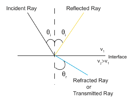
\[\frac{\sin \theta_i}{v_1}=\frac{\sin \theta_r}{v_2}\]
\(v_2>v_1\) is the most common interface in the earth, and \(\theta_r>\theta_i\) is due to \(v_2>v_1\).
Now that we've reviewed, let's first look at two sample ray paths.
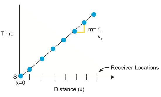
The direct wave travels horizontally along the surface. The Rs represent receiving stations. What is the arrival time at each station?

\[distance=velocity\cdot time\]
\[x=v_1\cdot t\]
Solve for t.
\[t=\frac{x}{v_1}\]
The above equation is the direct ray travel/arrival time. The equation is a line whose slope is \(\frac{1}{v_1}\) and intercept=0.
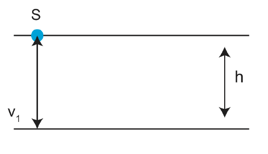
Using the vertical incidence of a reflected ray, we can derive an equation to calculate the time the ray took to reach the receiver:
\[d=v\cdot t\]
\[2h=v_1\cdot t\]
\[t=\frac{2h}{v_1}\]
Now, let's look at what happens as \(\theta_i\) increases.
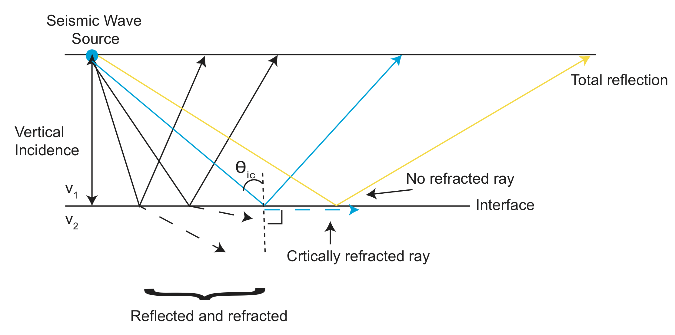
We can see from the figure that after the hammer blow/weight drop/small explosion (the seismic wave source), the waves go out in all directions. If there is a large angle reflection of a wave, all energy is reflected and none is refracted. This is called total reflection. When \(\theta_r\) increases until 90o, the wave is critically refracted. The critically refracted ray is crucial to surveys.
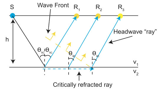
The critically refracted ray generates a 'head wave'. Receivers (R1, R2, R3) on the surface detect head wave at t1, t2, t3, which correspond with increasing distance from the source. We can use geometry and arrival times to determine v1, v2, and h. One of the cons of momentum and fitting boundary conditions is that it sends energy back into the top layer.
Now we're going to look at refraction geometry
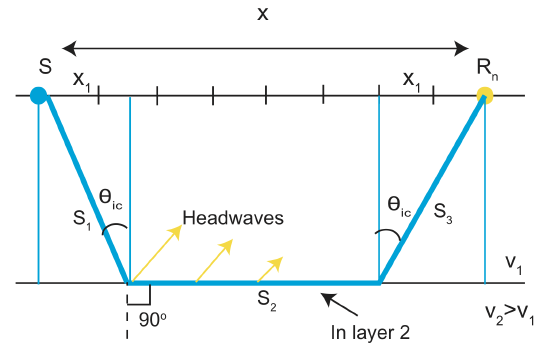
We know that
\[\frac{\sin\theta_{ic}}{v_1}=\frac{sin90^o}{v_2}\]
\[\sin\theta_{ic}=\frac{v_1}{v_2}\]
To get refraction, we must have v2>v1. Looking at the above figure, how do we figure out what are the distances s1, s2, and s3? What are velocities v1, v2, and v3? To get the travel time for each segment,
\[ \begin{align} [t &=t_1+t_2+t_3 \\[4pt] &=\frac{s_1}{v_1}+\frac{s_2}{v_2}+\frac{s_3}{v_3} \end{align}\]
We know that \(s_1=s_3\) so:
\[t=\frac{2s_1}{v_1}+s_2\]
Now we need to know 'what is s1'?
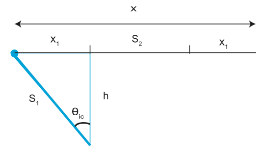
From the triangle we can derive that:
\[s_1=\frac{h}{\cos\theta_{ic}}\]
\[x_1=h\cdot \tan\theta_{ic}\]
\[s_2=x-2x_1\]
Substituting:
\[s_2=x-2h\cdot \tan\theta_{ic}\]
\[t=\frac{2h}{v_1\cos\theta_{ic}} +\frac{(x-2h\cdot \tan\theta_{ic})}{v_2}\]
We can use
\[\tan\theta_{ic}=\frac{\sin\theta_{ic}}{\cos\theta_{ic}}\]
We know that \(\sin\theta_{ic}=\frac{v_1}{v_2}\) from \(\frac{\sin\theta_{ic}}{v_1}=\frac{sin(90)}{v_2}\) and that \(sin^2\theta_{ic}+cos^2\theta_{ic}=1\)
\[t=\frac{x}{v_2}+\frac{2h(v^2_2-v^2_1)^{\frac{1}{2}}}{v_1v_2}\]
Or we can write it as
\[t=\frac{x}{v_1}+\frac{2h}{v_1}(1-\frac{v^2_1}{v^2_2})^{\frac{1}{2}}\]
So what kind of equation is this exactly? Its a line with slope \(m=\frac{1}{v_2}\) and \(t(o)=\frac{2h(v^2_2-v^2_1)^{\frac{1}{2}}}{v_1v_2}\)
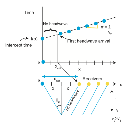
From Figure \(\PageIndex{9}\), we can also derive that
\[ \begin{align}x_{crit}=2x_1 \\[4pt] &=2h\cdot \tan\theta_{ic} \end{align}\]
Another important value that can be graphed is the crossover distance, or \(x_{co}\).
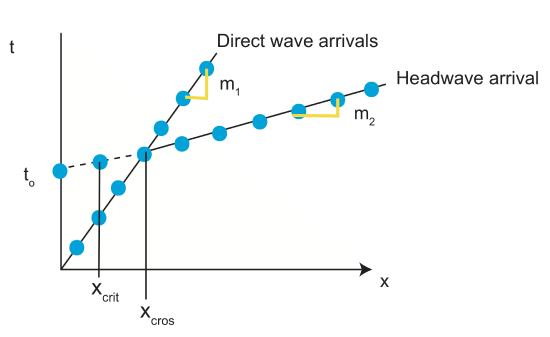
The xco is when the tdir=thead(rfr).
\[x_{co}=2h(\frac{v_2+v_1}{v_2-v_1})^{\frac{1}{2}}\]
To summarize what we learned in this section:
How do you determine subsurface structure?
- Identify direct wave arrivals
- Measure slope→m1
- Calculate v1(layer 1)→\(v_1=\frac{1}{m_1}\)
- Identify headwave arrivals
- Measure slope, m, intercept, to
- Calculate v2(layer 2)→\(v_2=\frac{1}{m_2}\)
- Use to, v1, and v2 to calculate h
- \(t_o=\frac{2h(v^2_2-v^2_1)^{\frac{1}{2}}}{v_1v_2}\)
- \(h=\frac{t_ov_1v_2}{2(v^2_2-v^2_1)^{\frac{1}{2}}}\)


