5.1: Basics of Wave Propagation

To understand some of the more complex aspects of seismology, we must first start at the beginning and get a handle on the basics of wave propagation. In this section, we will examine three primary concepts:

1. The Basics of Waves
2. Types of Seismic Waves
3. Optics: Reflection, Transmission (Refraction), and Snell's Law

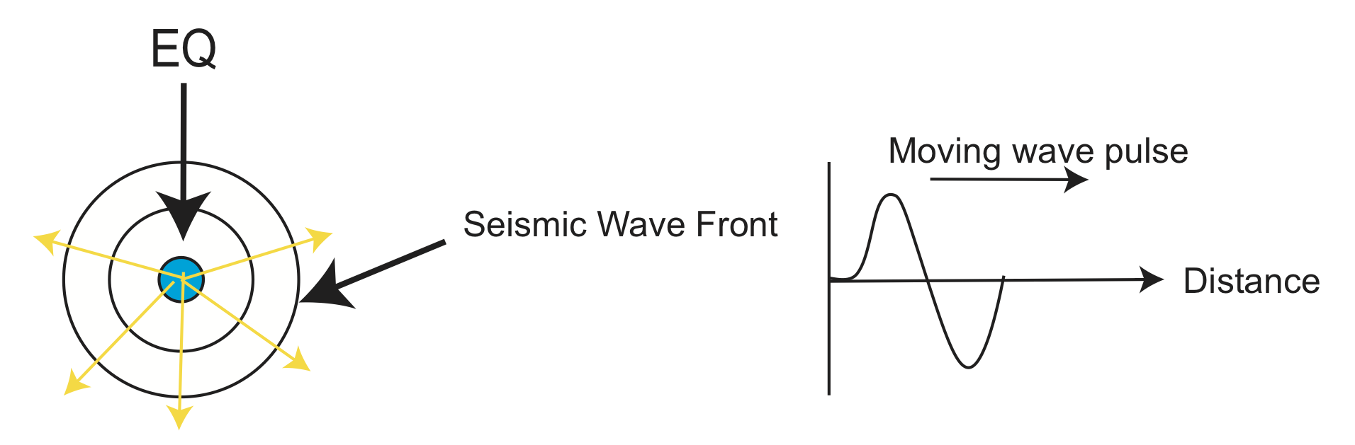
The Basics of Waves

Figure \(\PageIndex{1}\): Amplitude and Wavelength

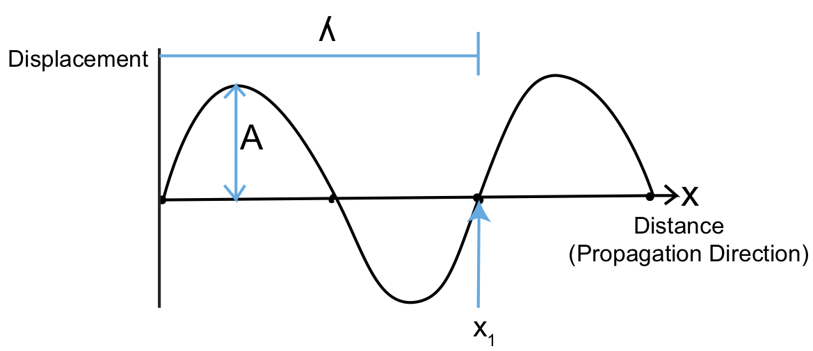
In the figure above, \(\lambda\) is the wavelength in meters and \(A\) is the amplitude in \(\mu m-cm\). If you were to stand at x₁ and watch the wave go by, you would see Figure \(\PageIndex{1}\):

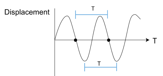where T is the period in s and \(f\) is the frequency in Hz. Frequency and period have the relation \(f=\frac{1}{T}\), and thus \(Hz=\frac{1}{s}\).

In terms of the relation between sound velocity and seismic velocity:

\[v=f\lambda\; \left[\dfrac{m}{s}\right]\]

Light has a similar relationship between frequency and wavelength,

\(c=f\lambda\), where different values for \(f\lambda\) give different colors of light.

Figure \(\PageIndex{2}\): Period

Types of Seismic Waves

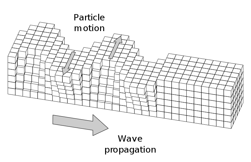
One category of seismic waves are body waves. Body waves are waves you have likely heard of before, P waves and S waves. P waves act like an accordion, and move parallel to the propagation direction.

Figure \(\PageIndex{3}\): Plane P-wave (CC BY-SA 3.0; Christophe Dang Ngoc Chan (cdang) via Wikimedia)

S waves can have two components of motion, vertical and horizontal. Most S waves usually have both components, S-vert and S-horiz, which can be polarized.

Figure \(\PageIndex{4}\): Plane S-wave (CC BY-SA 3.0; Christophe Dang Ngoc Chan (cdang) via Wikimedia)

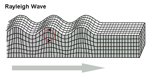
The other category of seismic waves are surface waves, which decay with depth. Thus, as the name suggests, they are the strongest at the surface. There are two main surface waves, Love waves and Rayleigh waves. Love waves have particle motion like that of the S-H component.

Figure \(\PageIndex{5}\): Love wave (CC BY 4.0; Nicoguaro via Wikimedia)

Rayleigh waves have the components of a P wave and a S-V wave. The particle motion is retrograde.

Figure \(\PageIndex{6}\): Rayleigh wave (Public Domain; Starmenclock via Wikimedia).

How fast do these waves actually move? Wave speed depends on two things, the density of the material the waves are traveling through and the elastic constant or 'stiffness'. Density is key to wave speed because the wave has to move mass. Imagine moving two materials in a wave-like pattern, a string and a metal cable. It takes more energy to move the more massive metal cable than it does the string because the cable is much denser. To understand the elastic constant, imagine moving a yarn and a stiff rope. In the yarn, it is hard to get the wave to move because the material lacks stiffness. With these two properties, we can write a relationship for wave velocity:

\[v\propto\frac{\text{Elastic constant}}{\text{Density}}\]

As v\(\uparrow\), \(\rho\downarrow\), the elastic constant \(\uparrow\).

Additional useful relationships when dealing with stress-strain due to seismic waves are

\[\sigma=E\epsilon\]

where \(E\) is Young's modulus that we discussed in Chapter 1.

\[F=-k\Delta x\]

Where \(k\) is the spring constant.

\[\nu=\frac{\epsilon_1}{\epsilon_3}\]

In addition to stress-strain deformation, we also have shear deformation.

Figure \(\PageIndex{7}\): Shear Deformation Variables

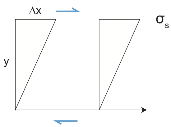
\[\epsilon_s=\frac{1}{2}\frac{\Delta x}{y}\]

\[\sigma_s=2G\epsilon_s\]

where \(G\) is the shear modulus.

\[G=\frac{\sigma_s}{2\epsilon_s}\left[\frac{N}{m^2}\right]\]

For reference, sometimes the shear modulus is represented by \(\mu\).

We can also have volumetric strain.

Figure \(\PageIndex{8}\): Volumetric Strain

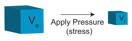
\[\frac{\Delta V}{V}=\frac{V_f-V_o}{V_o}\]

\[P=\kappa\frac{\Delta V}{V}\]

Where \(\kappa\) is the bulk Modulus

\[\kappa=\frac{P}{(\frac{\Delta V}{V})}[\frac{N}{m^2}]\]

To summarize and review some of the constants that we have learned so far:

• E-Young's Modulus (elongation dilation)
• \(\nu\)-Poisson's Ratio (compensation deformation)
• G or \(\mu\) - shear muodulus
• \(\kappa\)- bulk modulus

In seismic calculations, you can use one set (E and \(\nu\)) or the other (G and \(\kappa\)).

Now let's learn how to actually calculate seismic velocities. For P-waves:

\[v_p=\sqrt{\frac{\kappa+\frac{4}{3}G}{\rho}}\;or\;\sqrt{\frac{E}{\rho}\frac{(1-\nu)}{(1-2\nu)(1+\nu)}}\]

For S-waves, we can calculate velocity as:

\[v_s=\sqrt{\frac{G}{\rho}}\;or\;\sqrt{\frac{E}{\rho}\frac{1}{(2(1+\nu))}}\]

To find the ratio of P and S-wave velocities:

\[\frac{v_p}{v_s}=\sqrt{\frac{2(1-\nu)}{(1-2\nu)}}\]

Thus, we can see that this only depends on \(\nu\). This ratio is a good indicator of gas/liquids in exploration geology

• \(\frac{v_p}{v_s}<2\) indicates gas+sand
• \(\frac{v_p}{v_s}>2\) indicates sand only

In general, we find that v_p~1.7v_s (~50% faster).

Unfortunately, for surface waves, we cannot easily write down equations for \(v_R\) and \(v_L\) because of depth dependence. Thus, to determine their velocity, we must solve the wave equation with boundary conditions.

Optics: Reflection, Transmission (Refraction), and Snell's Law

Figure \(\PageIndex{9}\): Seismic Wave Front Model

We can use the ray path to think about what happens to a wave when it encounters a boundary.

Figure \(\PageIndex{10}\): Wave Fronts

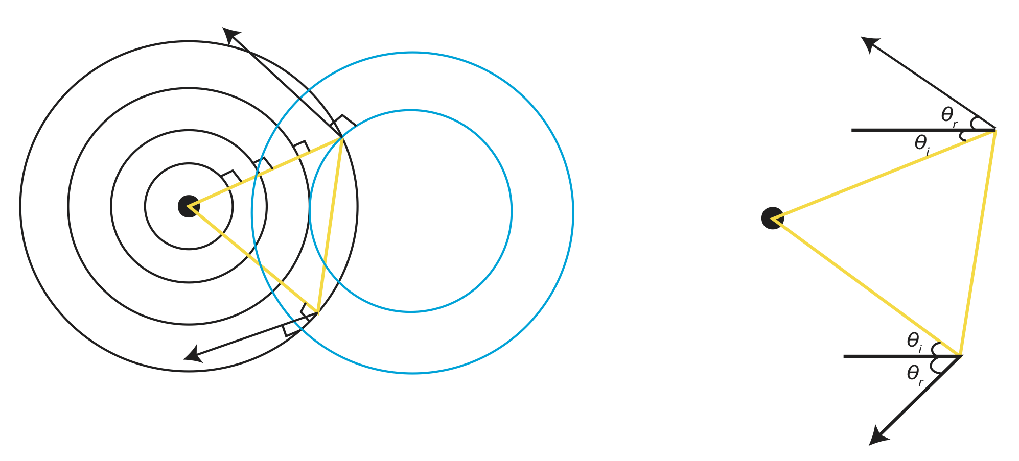
The most important information you can take from the above figure is that \(\theta_i=\theta_r\), i.e. the angle of incidence=the angle of reflection. We've now considered reflection of waves, but what about refraction?

Figure \(\PageIndex{11}\): Refraction

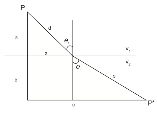
\[T_{p-p'}=\frac{d}{v_1}+\frac{e}{v_1}=\frac{\sqrt{a^2+x^2}}{v_1}+\frac{\sqrt{b^2+(c-x)^2}}{v_2}\]

Fermat's Principle of least time states that the ray will follow the path that takes the shortest time. We can use this principle to derive one of the most important laws in seismology, Snell's Law.

\[\begin{align*} \frac{dT}{dx}=0 \\[4pt] &=\frac{x}{v_1\sqrt{a^2+x^2}}-\frac{(c-x)}{v_2\sqrt{b^2+(c-x)^2}} \end{align*}\]

where \(\sin \theta_i=\frac{x}{\sqrt{a^2+x^2}}\) and \(\sin \theta_r=\frac{(c-x)}{\sqrt{b^2+(c-x)^2}}\)

Now we can rewrite the equation as:

\[\frac{dT}{dx}=\frac{\sin \theta_i}{v_1}-\frac{\sin \theta_r}{v_2}\]

\[\frac{\sin \theta_i}{v_1}=\frac{\sin \theta_r}{v_2}\]

The above equation is Snell's Law. To better understand Fermat's Principle and why a ray takes the path of shortest time, we can also say that \(\frac{\sin \theta_i}{v_1}\)=p=slowness. This slowness is constant along a ray path.

Figure \(\PageIndex{12}\): Curving Ray Path

\[\frac{sin(i)}{v}=constant=p\]

The ray path curves to adjust for changing velocity between different mediums. Thus, the ray takes the shortest time path. Let's now take a better look at Snell's Law, what it tells us, and what makes it so useful.

Figure \(\PageIndex{13}\): Reflection vs. Refraction

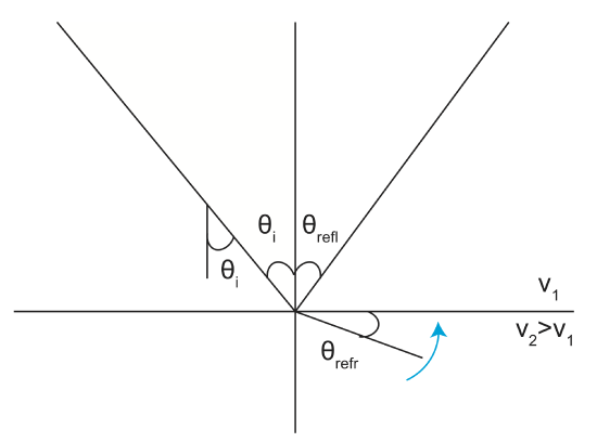
The figure shows the difference between reflection and refraction when a ray encounters a boundary.

\[\frac{\sin \theta_i}{v_1}=\frac{\sin \theta_{refr}}{v_2}\]

If we keep increasing v₂, \(\theta_r\) increases up to 90^o. At 90^o, we have critical refraction, where \(sin(90^o)=1\). Plugging this into Snell's Law we get:

\[\frac{\sin \theta_i}{v_1}=\frac{1}{v_2}\]

\[\theta_{ic}=sin^{-1}(\frac{v_1}{v_2})\]

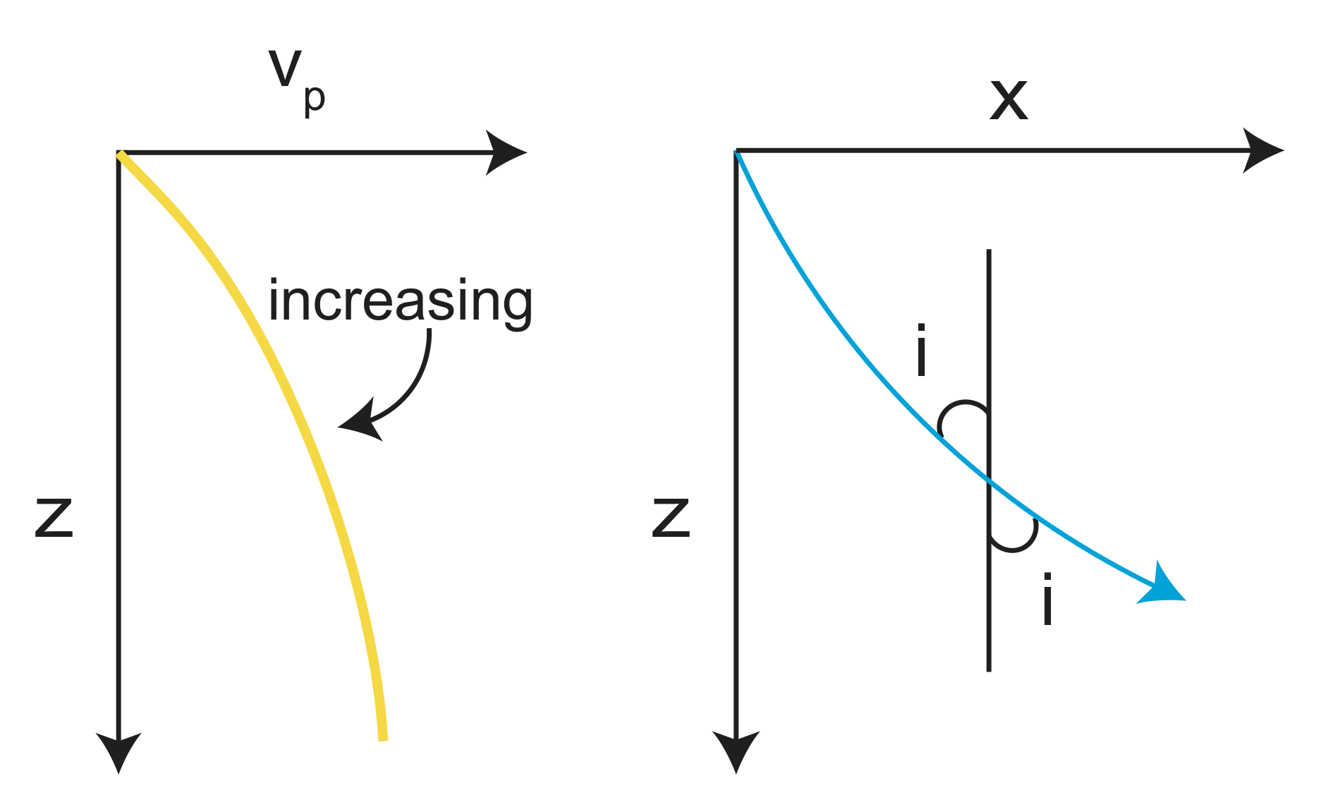
If \(\theta_{ir}>\theta_{ic}\), we get total reflection. What does Snell's Law actually tell us? (slowness)

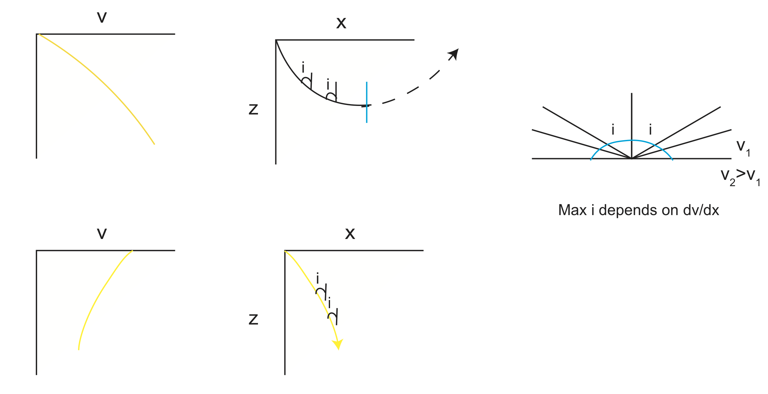
v increases with depth, i increases.

v decreases with depth, i decreases.

Figure \(\PageIndex{14}\): Changes in i with respect to v