4.5: Relative Velocity and Reference Frames
- Page ID
- 3735
\( \newcommand{\vecs}[1]{\overset { \scriptstyle \rightharpoonup} {\mathbf{#1}} } \)
\( \newcommand{\vecd}[1]{\overset{-\!-\!\rightharpoonup}{\vphantom{a}\smash {#1}}} \)
\( \newcommand{\id}{\mathrm{id}}\) \( \newcommand{\Span}{\mathrm{span}}\)
( \newcommand{\kernel}{\mathrm{null}\,}\) \( \newcommand{\range}{\mathrm{range}\,}\)
\( \newcommand{\RealPart}{\mathrm{Re}}\) \( \newcommand{\ImaginaryPart}{\mathrm{Im}}\)
\( \newcommand{\Argument}{\mathrm{Arg}}\) \( \newcommand{\norm}[1]{\| #1 \|}\)
\( \newcommand{\inner}[2]{\langle #1, #2 \rangle}\)
\( \newcommand{\Span}{\mathrm{span}}\)
\( \newcommand{\id}{\mathrm{id}}\)
\( \newcommand{\Span}{\mathrm{span}}\)
\( \newcommand{\kernel}{\mathrm{null}\,}\)
\( \newcommand{\range}{\mathrm{range}\,}\)
\( \newcommand{\RealPart}{\mathrm{Re}}\)
\( \newcommand{\ImaginaryPart}{\mathrm{Im}}\)
\( \newcommand{\Argument}{\mathrm{Arg}}\)
\( \newcommand{\norm}[1]{\| #1 \|}\)
\( \newcommand{\inner}[2]{\langle #1, #2 \rangle}\)
\( \newcommand{\Span}{\mathrm{span}}\) \( \newcommand{\AA}{\unicode[.8,0]{x212B}}\)
\( \newcommand{\vectorA}[1]{\vec{#1}} % arrow\)
\( \newcommand{\vectorAt}[1]{\vec{\text{#1}}} % arrow\)
\( \newcommand{\vectorB}[1]{\overset { \scriptstyle \rightharpoonup} {\mathbf{#1}} } \)
\( \newcommand{\vectorC}[1]{\textbf{#1}} \)
\( \newcommand{\vectorD}[1]{\overrightarrow{#1}} \)
\( \newcommand{\vectorDt}[1]{\overrightarrow{\text{#1}}} \)
\( \newcommand{\vectE}[1]{\overset{-\!-\!\rightharpoonup}{\vphantom{a}\smash{\mathbf {#1}}}} \)
\( \newcommand{\vecs}[1]{\overset { \scriptstyle \rightharpoonup} {\mathbf{#1}} } \)
\( \newcommand{\vecd}[1]{\overset{-\!-\!\rightharpoonup}{\vphantom{a}\smash {#1}}} \)
\(\newcommand{\avec}{\mathbf a}\) \(\newcommand{\bvec}{\mathbf b}\) \(\newcommand{\cvec}{\mathbf c}\) \(\newcommand{\dvec}{\mathbf d}\) \(\newcommand{\dtil}{\widetilde{\mathbf d}}\) \(\newcommand{\evec}{\mathbf e}\) \(\newcommand{\fvec}{\mathbf f}\) \(\newcommand{\nvec}{\mathbf n}\) \(\newcommand{\pvec}{\mathbf p}\) \(\newcommand{\qvec}{\mathbf q}\) \(\newcommand{\svec}{\mathbf s}\) \(\newcommand{\tvec}{\mathbf t}\) \(\newcommand{\uvec}{\mathbf u}\) \(\newcommand{\vvec}{\mathbf v}\) \(\newcommand{\wvec}{\mathbf w}\) \(\newcommand{\xvec}{\mathbf x}\) \(\newcommand{\yvec}{\mathbf y}\) \(\newcommand{\zvec}{\mathbf z}\) \(\newcommand{\rvec}{\mathbf r}\) \(\newcommand{\mvec}{\mathbf m}\) \(\newcommand{\zerovec}{\mathbf 0}\) \(\newcommand{\onevec}{\mathbf 1}\) \(\newcommand{\real}{\mathbb R}\) \(\newcommand{\twovec}[2]{\left[\begin{array}{r}#1 \\ #2 \end{array}\right]}\) \(\newcommand{\ctwovec}[2]{\left[\begin{array}{c}#1 \\ #2 \end{array}\right]}\) \(\newcommand{\threevec}[3]{\left[\begin{array}{r}#1 \\ #2 \\ #3 \end{array}\right]}\) \(\newcommand{\cthreevec}[3]{\left[\begin{array}{c}#1 \\ #2 \\ #3 \end{array}\right]}\) \(\newcommand{\fourvec}[4]{\left[\begin{array}{r}#1 \\ #2 \\ #3 \\ #4 \end{array}\right]}\) \(\newcommand{\cfourvec}[4]{\left[\begin{array}{c}#1 \\ #2 \\ #3 \\ #4 \end{array}\right]}\) \(\newcommand{\fivevec}[5]{\left[\begin{array}{r}#1 \\ #2 \\ #3 \\ #4 \\ #5 \\ \end{array}\right]}\) \(\newcommand{\cfivevec}[5]{\left[\begin{array}{c}#1 \\ #2 \\ #3 \\ #4 \\ #5 \\ \end{array}\right]}\) \(\newcommand{\mattwo}[4]{\left[\begin{array}{rr}#1 \amp #2 \\ #3 \amp #4 \\ \end{array}\right]}\) \(\newcommand{\laspan}[1]{\text{Span}\{#1\}}\) \(\newcommand{\bcal}{\cal B}\) \(\newcommand{\ccal}{\cal C}\) \(\newcommand{\scal}{\cal S}\) \(\newcommand{\wcal}{\cal W}\) \(\newcommand{\ecal}{\cal E}\) \(\newcommand{\coords}[2]{\left\{#1\right\}_{#2}}\) \(\newcommand{\gray}[1]{\color{gray}{#1}}\) \(\newcommand{\lgray}[1]{\color{lightgray}{#1}}\) \(\newcommand{\rank}{\operatorname{rank}}\) \(\newcommand{\row}{\text{Row}}\) \(\newcommand{\col}{\text{Col}}\) \(\renewcommand{\row}{\text{Row}}\) \(\newcommand{\nul}{\text{Nul}}\) \(\newcommand{\var}{\text{Var}}\) \(\newcommand{\corr}{\text{corr}}\) \(\newcommand{\len}[1]{\left|#1\right|}\) \(\newcommand{\bbar}{\overline{\bvec}}\) \(\newcommand{\bhat}{\widehat{\bvec}}\) \(\newcommand{\bperp}{\bvec^\perp}\) \(\newcommand{\xhat}{\widehat{\xvec}}\) \(\newcommand{\vhat}{\widehat{\vvec}}\) \(\newcommand{\uhat}{\widehat{\uvec}}\) \(\newcommand{\what}{\widehat{\wvec}}\) \(\newcommand{\Sighat}{\widehat{\Sigma}}\) \(\newcommand{\lt}{<}\) \(\newcommand{\gt}{>}\) \(\newcommand{\amp}{&}\) \(\definecolor{fillinmathshade}{gray}{0.9}\)Reference Frames, Relative and Absolute Plate Velocity
Relative velocity is the velocity with respect to some frame of reference. Considering the relative motion of plates, the reference frame can be something external (like the location of rising plumes from the core mantle boundary) or it can be one of the plates, or even a plate boundary. The reference frame is set by the object that is being held fixed. In other words it is the object that the velocities are measure with respect to.
If you have two plates, A and B, the velocity of plate B relative to plate A is denoted by \(_AV_B\), where the first subscript is the fixed plate (A) and the second subscript is the moving plate (B). The relative motion is calculated as:
\[_AV_B = V_B - V_A \]
Note that you subtract the velocity of the fixed plate from the moving plate. Similarly, we can reverse which plate is being held fixed and hold plate B fixed. Then:
\[_BV_A = V_A - V_B \]
gives the velocity of plate A relative to plate B.
As an example, take \(V_A = 60\) mm/yr and \(V_B = 20\) mm/yr, then
\[_AV_B = 20 - 60 = -40 \]
\[_BV_A = 60 - 20 = 40 \]
Note that \(_AV_B = -40 \) mm/yr and \(_BV_A = 40\) mm/yr, so
\[_AV_B = - _BV_A\]
The magnitude of the motion between the two plates is the same (40 mm/y in the example): this is the relative velocity, which does depend on which plate I choose as the reference frame. The sign, however does depend on which plate is being used as the reference frame, and indicates direction of relative motion.
Finally, if an external reference frame is being used, then we may refer to the motion of a plate as an absolute plate velocity. This indicates that the plate velocity is not the relative motion between two plates, but rather it is the motion of each plate relative to the external frame of reference (e.g., the lighthouse in the example below). The relative motion of the two plates, can be found by differencing the absolute plate velocities (see example below).
Example Relative Velocity
To better understand relative velocity, consider a simple example of people on a ship.
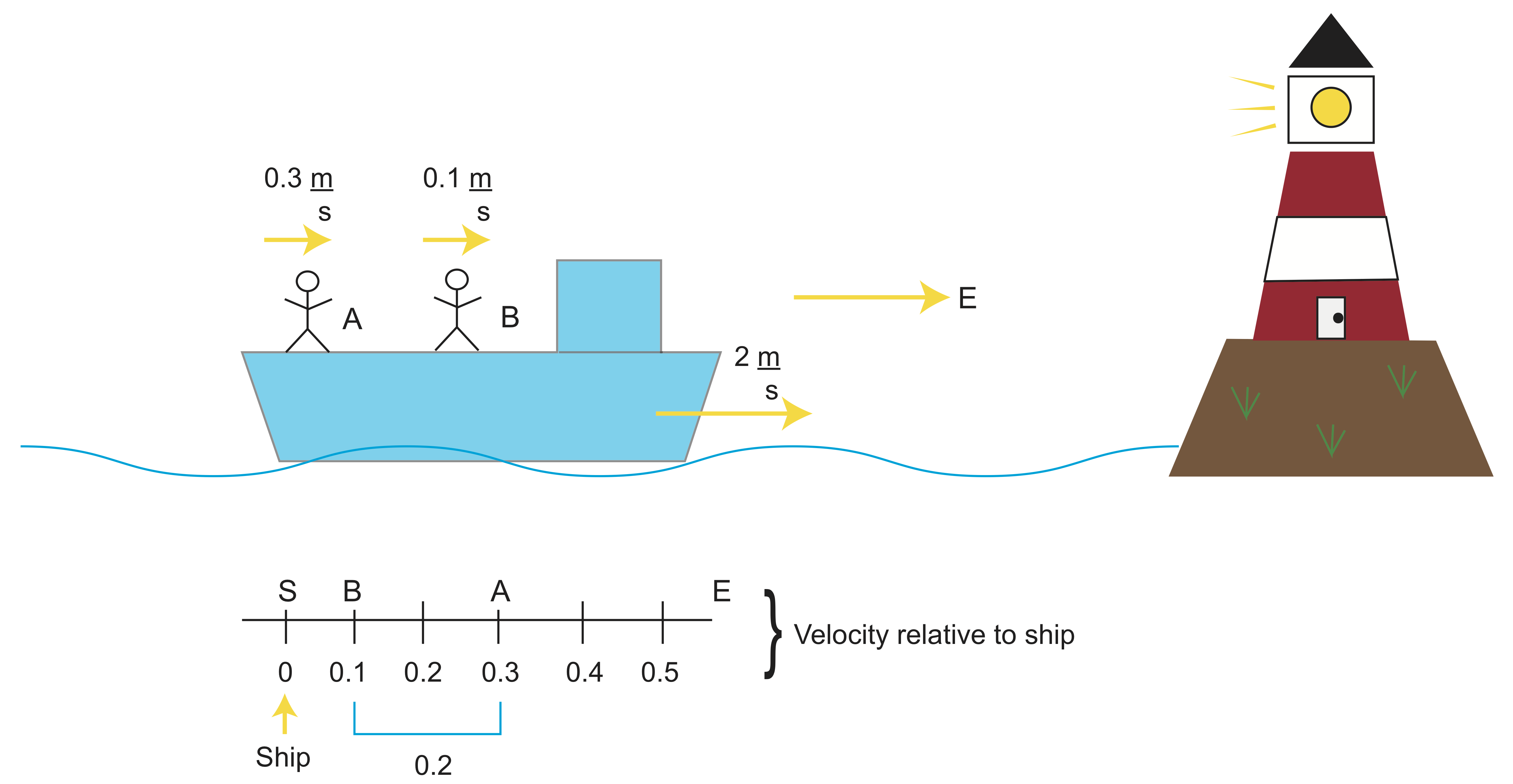
The velocity line indicates velocity relative to the ship.
We want to know 'how fast is person A approaching person B'? Another way to phrase this is "the motion of person B relative to person A". Translating these words to an algebraic expression we get:
\[\begin{align*}_AV_B &=V_A-V_B \\[4pt] &=0.2\frac{m}{s} \\[4pt] &=0.3-0.1 \end{align*}\]
Now we want to know, "how fast are the people moving towards the lighthouse"?
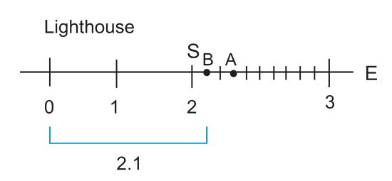
\[_LV_B=_LV_S+_SV_B\]
The two "S" cancel, and the "L" indicates movement relative to the lighthouse.
\[\begin{align*} _LV_B&=2.0+.01 \\[4pt] &=2.1 \end{align*}\]
2.1 is the "absolute velocity"
Now what if person A turns around and starts walking the other way? We want to know 'what is AVB'?

How do we make VA=0? ⇒ Add to 0.3. We now know that VA=-0.3.
\[_AV_B=_SV_B-_SV_A\]
\[_SV_A=-_AV_S\]
\[_AV_B=_AV_S+_SV_B\]
Once again the "S" cancel.
\[_AV_B=0.3+0.1\]
\[_AV_B=0.4\]
One final question, what is the motion of person A relative to the lighthouse?
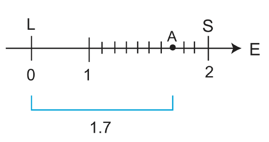
\[_LV_A=_LV_S+_SV_B\]
Where LVA indicates the absolute velocity or velocity relative to L, and sVB is the relative velocity.
\[_LV_B=2.0+(-0.3)\]
\[_LV_B=1.7\]
Relative Velocity Between Plates
So now let's try this with plates. Consider again our two plate system with plate A diverging away from plate B perpendicular to the boundary between the two plates. We assume plate B is not moving (i.e. plate B is fixed). The velocity of plate A relative to plate B is denoted \( _BV_A \). If instead we wanted to hold plate A fixed and consider plate B moving away from plate, then this would be denoted \( _AV_B \). As a way to remember this nomenclature, note: \( _{fixed} V _{moving} \).
Calculating Relative Plate Velocity
With the age of the plate adjacent to the spreading ridge determined from magnetic anomalies, we can calculate the relative velocity from the distance \(\Delta x\) between the spreading ridge and the edge (start or end) of a dated magnetic anomaly with age \( t_a\) as
\[ _AV_B = \frac{\Delta x}{t_a}\]
Let's say the age is 5 my and the distance is 100 km. Then, in this case,
\[ _AV_B = \frac{-100\,\mathrm{km}}{5\,\mathrm{ my}} = -20\,\mathrm{km/my} = -20\,\mathrm{mm/y} = -2\,\mathrm{cm/y} \]
We consider velocity in the negative x direction to be negative, and velocity in the positive direction to be positive. Therefore, the motion of plate B (in the positive direction) relative to plate A is \(_BV_A = + 2\,\mathrm{cm/yr}\) Notice that when we choose to hold a plate fixed, the spreading center necessarily moves as both plates grow symmetrically during the spreading process. The spreading center moves away from the plate being held fixed.
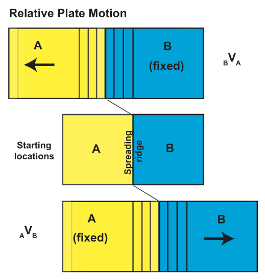
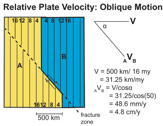
When the diverging motion of the plates is perpendicular to the spreading center, then the relative velocity of the two plates is the same as the spreading rate. However, the motion of the plate need not be perpendicular to the plate boundary. In this case, the magnetic anomalies still form parallel to the spreading center, but calculating the relative motion must take into account the distance between anomalies in the direction of spreading. The direction (orientation) of spreading relative to the spreading center can be determined by the orientation of transform faults between ridge segments. The transform faults are active faults between the ridge segments and are parallel to the relative plate motion. Beyond the ridge segments, the previous location of the transform fault is recorded as a topographic feature called a fracture zone. There is no relative motion across the fracture zone, it resides wholly within the plate on that side of the spreading center. When a transform fault or fracture zone indicates oblique spreading, the relative velocity can be determined by first calculating the apparent velocity perpendicular to the ridge, \( V \) and then correcting for the actual orientation of the plate motion given by the angle between the perpendicular direction and the actual plate motion direction \( \alpha \) and is given by
\[ _AV_B = \frac{V}{\cos \alpha} \]
Reference Frames
In the above example we arbitrarily hold one of the plates fixed and calculate the relative velocity between the two plates. However, one could imagine holding the spreading center fixed or some other external reference frame. In considering the motion of tectonic plates there is not an obvious choice for the reference frame, because the plate are moving above a mantle that is dynamically mixing and changing in time. At one time it was thought that the plumes feeding hot-spot volcanoes might serve as a fixed reference frame if these plumes originate at the core-mantle boundary and then rise through the mantle without being entrained by the flow in the mantle. Locally and for short periods of time this assumption appears true, but globally the plumes move relative to each other and simulations show that their origination point can move through time. Therefore, different research groups make different choices about which reference frame to use depending on the question they are asking... e.g., is it about recent plate motions, or does the physical interpretation depend on the absolute motion of the plate. It is therefore also useful to be comfortable with changing reference frame as needed.
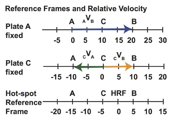
First, it is important to note that that relative plate velocity does not depend on choice of reference frame. We saw this above when we changed from a fixed-plate-A reference frame to a fixed-plate-B reference frame. Consider again the two plate A and B diverging at a spreading ridge with \( _A V_B = +20\) cm/y. Now, consider that Plate A is in fact subducting under Plate C with \( _C V_A = -10\) cm/y (note plate C is now fixed). Then, what is the relative velocity between Plate B and Plate C?
The Velocity Line
One way to consider this question is using a velocity line. First choose which plate to hold fixed. Let's hold plate A fixed. Then \( _A V_C = +10\) cm/y and \( _A V_B = +20\) cm/y. To determine the relative velocity between Plate B and Plate C, we need to hold one of these plates fixed. Let's hold plate C fixed. On the velocity line, we do this by subtracting the velocity of plate C from all the points, so it now lies at the origin and is fixed. The relative velocity of plate C with respect to plate B can then be read from the velocity line, \( _C V_B = +10\) cm/y. Therefore, regardless of the which plate is held fixed (the reference frame), the relative velocity between to plate is always just the difference in the velocity of the two plates (expressed in the same reference frame). As one last example, consider that instead of holding any of the plates fixed, we wanted to use a "hot-spot" reference frame. Plate A is moving -15 cm/y with respect to the the hot-spot reference frame. The velocity of each of the plate can be adjusted by subtracting 5 cm/y. In the hot-spot reference frame all the plate are moving with some velocity and their absolute velcoity have all shifted compared to the fixed plate reference frames. However, the relative velocities remain the same.
The Velocity Plane
Unlike the example above in which all the plates are moving a long a single direction (one-dimensional, 1D motion), plates actually move in two-dimensions (either on a plate or the surface of a sphere). Therefore, to consider relative plate motions and reference frames, we need to deal with the plate velocity as a vector that has both a magnitude and a direction. As our reference coordinate system, we use the east-west direction east is positive) and the north-south direction (north is positive). The velocity of a plate is then given by its speed V, and its direction, \(\theta\), an angle measured clockwise from north: these are polar coordinate \((r,\theta\)). The Cartesian components of motion of the plate in the north and south directions are then given by:
\[ V^E = V \sin (\theta) \]
\[V^N = V \cos (\theta) \]
The polar coordinates can also be determined from the Cartesian components as:
\[V = \sqrt{{V^E}^2 + {V^N}^2} \]
\[ \theta = \tan^{-1} (V^E/V^N) \]
Finding Relative Plate Motion in 2D
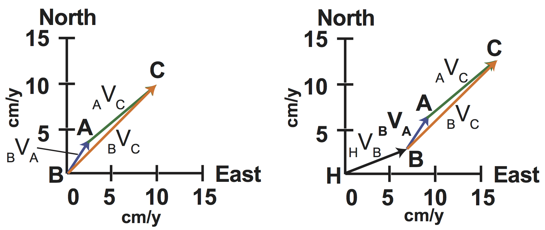
The relative motion of plates in 2D can then be found by adding the components in Cartesian coordinates, and the converting the result to polar coordinates if desired. For example, if the motion of plate A with respect to plate B is given by \( _BV_A = 5\) cm/y, \(\theta_{BA} = 30^\circ \) and the plate motion of plate C with respect to plate A is given by \( _AV_C = 10\) cm/y, \(\theta_{AC} = 50^\circ \), then we first convert both velocities to Cartersian coordinates.
Plate B-A:
\[ _BV_A^E = _BV_A \sin (\theta_{BA} = 5 \sin(30) = 2.5 \,\mathrm{ cm/y} \]
\[ _BV_A^N = _BV_A \sin (\theta_{BA} = 5 \cos(30) = 4.33 \,\mathrm{ cm/y} \]
Plate A-C:
\[ _AV_C^E = _AV_C \sin (\theta_{AC} = 10 \sin(50) = 7.66\, \mathrm{ cm/y} \]
\[ _AV_C^N = _AV_C \sin (\theta_{AC} = 10 \cos(50) = 6.42\, \mathrm{ cm/y} \]
Next, we add the north components together and the east components together :
\[_BV_C^N = _BV_A^N + _AV_C^N = 4.33 + 6.42 = 10.75\, \mathrm{ cm/y}\]
\[_BV_C^E = _BV_A^E + _AV_C^E = 2.5 + 7.66 = 10.16\, \mathrm{ cm/y}\]
and then convert back to polar coordinates:
\[_BV_C = \sqrt{{_BV_C^E}^2 + {_BV_C^N}^2} = \sqrt{ 10.75^2 + 10.16^2} = 14.79\, \mathrm{ cm/y}\]
\[ \theta_{BC} = \tan^{-1} (_BV_C^E/_BV_C^N) = \tan^{-1} (10.16/10.75) = 43.38^\circ \]
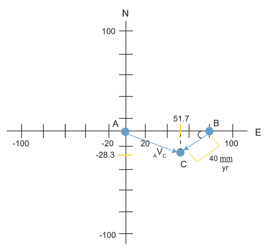
This process of adding plate velocity vectors can also be illustrated on a velocity plane. Similar to the velocity line the axis represent components of velocity in North and East directions. The velocity vectors are added by drawing the velocity vectors in the appropriate direction and magnitude. In the case describe above, we first draw the velocity of Plate A relative to Plate B. Therefore, Plate B is fixed and is located at the origin. Next, we draw the velocity of Plate C relative to A. In this case, the origin of the vector is the located at the point marked A (the point having the velocity components of Plate A relative to Plate B. The velocity of Plate C is then determined by drawing the vector that closes the velocity triangle, going from point B (fixed) to plate C. Also similar to the a change in reference frame on the velocity line, a change in reference frame in 2-D simply translate the velocity vectors within the velocity plate. Therefore, again, the relative velocities stay the same, by the absolute velocity magnitude depend on which reference frame is used.
Let's now reverse the procedure. We are going to try determining the velocity diagram from plate boundaries.
Determining the Velocity Diagram From Plate Boundaries.
We are going to look at the motion of plate C with respect to plate A.
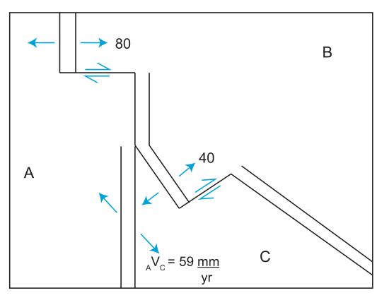
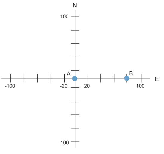
1.Hold A fixed (Because we have AVB)→plot at origin. We could also hold B fixed because we have BVA and BVC.
2. B moves east at 80\(\frac{mm}{yr}\) with respect to A.
AVB=80\(\frac{mm}{yr}\)
3. C moves southwest (45o) from B at 40\(\frac{mm}{yr}\)
E=40cos45o=28.3
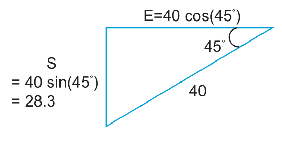
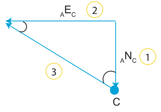
\[_AN_C=-28.3\]
\[_AE_C=_AE_B+_BE_C\]
\[_AE_C=80+(-28.3)\]
\[_AE_C=51.7\]
\[_AV_C=\sqrt{(51.7)^2+(28.3)^2}\]
\[_AV_C=58.9\]
\[_AV_C\approx 59\]
Now that we have our velocities, we can place them on the velocity graph.
