
4.2: Magnetic Anomalies on the Seafloor
- Page ID
- 3514

\( \newcommand{\vecs}[1]{\overset { \scriptstyle \rightharpoonup} {\mathbf{#1}} } \)
\( \newcommand{\vecd}[1]{\overset{-\!-\!\rightharpoonup}{\vphantom{a}\smash {#1}}} \)
\( \newcommand{\id}{\mathrm{id}}\) \( \newcommand{\Span}{\mathrm{span}}\)
( \newcommand{\kernel}{\mathrm{null}\,}\) \( \newcommand{\range}{\mathrm{range}\,}\)
\( \newcommand{\RealPart}{\mathrm{Re}}\) \( \newcommand{\ImaginaryPart}{\mathrm{Im}}\)
\( \newcommand{\Argument}{\mathrm{Arg}}\) \( \newcommand{\norm}[1]{\| #1 \|}\)
\( \newcommand{\inner}[2]{\langle #1, #2 \rangle}\)
\( \newcommand{\Span}{\mathrm{span}}\)
\( \newcommand{\id}{\mathrm{id}}\)
\( \newcommand{\Span}{\mathrm{span}}\)
\( \newcommand{\kernel}{\mathrm{null}\,}\)
\( \newcommand{\range}{\mathrm{range}\,}\)
\( \newcommand{\RealPart}{\mathrm{Re}}\)
\( \newcommand{\ImaginaryPart}{\mathrm{Im}}\)
\( \newcommand{\Argument}{\mathrm{Arg}}\)
\( \newcommand{\norm}[1]{\| #1 \|}\)
\( \newcommand{\inner}[2]{\langle #1, #2 \rangle}\)
\( \newcommand{\Span}{\mathrm{span}}\) \( \newcommand{\AA}{\unicode[.8,0]{x212B}}\)
\( \newcommand{\vectorA}[1]{\vec{#1}} % arrow\)
\( \newcommand{\vectorAt}[1]{\vec{\text{#1}}} % arrow\)
\( \newcommand{\vectorB}[1]{\overset { \scriptstyle \rightharpoonup} {\mathbf{#1}} } \)
\( \newcommand{\vectorC}[1]{\textbf{#1}} \)
\( \newcommand{\vectorD}[1]{\overrightarrow{#1}} \)
\( \newcommand{\vectorDt}[1]{\overrightarrow{\text{#1}}} \)
\( \newcommand{\vectE}[1]{\overset{-\!-\!\rightharpoonup}{\vphantom{a}\smash{\mathbf {#1}}}} \)
\( \newcommand{\vecs}[1]{\overset { \scriptstyle \rightharpoonup} {\mathbf{#1}} } \)
\( \newcommand{\vecd}[1]{\overset{-\!-\!\rightharpoonup}{\vphantom{a}\smash {#1}}} \)
\(\newcommand{\avec}{\mathbf a}\) \(\newcommand{\bvec}{\mathbf b}\) \(\newcommand{\cvec}{\mathbf c}\) \(\newcommand{\dvec}{\mathbf d}\) \(\newcommand{\dtil}{\widetilde{\mathbf d}}\) \(\newcommand{\evec}{\mathbf e}\) \(\newcommand{\fvec}{\mathbf f}\) \(\newcommand{\nvec}{\mathbf n}\) \(\newcommand{\pvec}{\mathbf p}\) \(\newcommand{\qvec}{\mathbf q}\) \(\newcommand{\svec}{\mathbf s}\) \(\newcommand{\tvec}{\mathbf t}\) \(\newcommand{\uvec}{\mathbf u}\) \(\newcommand{\vvec}{\mathbf v}\) \(\newcommand{\wvec}{\mathbf w}\) \(\newcommand{\xvec}{\mathbf x}\) \(\newcommand{\yvec}{\mathbf y}\) \(\newcommand{\zvec}{\mathbf z}\) \(\newcommand{\rvec}{\mathbf r}\) \(\newcommand{\mvec}{\mathbf m}\) \(\newcommand{\zerovec}{\mathbf 0}\) \(\newcommand{\onevec}{\mathbf 1}\) \(\newcommand{\real}{\mathbb R}\) \(\newcommand{\twovec}[2]{\left[\begin{array}{r}#1 \\ #2 \end{array}\right]}\) \(\newcommand{\ctwovec}[2]{\left[\begin{array}{c}#1 \\ #2 \end{array}\right]}\) \(\newcommand{\threevec}[3]{\left[\begin{array}{r}#1 \\ #2 \\ #3 \end{array}\right]}\) \(\newcommand{\cthreevec}[3]{\left[\begin{array}{c}#1 \\ #2 \\ #3 \end{array}\right]}\) \(\newcommand{\fourvec}[4]{\left[\begin{array}{r}#1 \\ #2 \\ #3 \\ #4 \end{array}\right]}\) \(\newcommand{\cfourvec}[4]{\left[\begin{array}{c}#1 \\ #2 \\ #3 \\ #4 \end{array}\right]}\) \(\newcommand{\fivevec}[5]{\left[\begin{array}{r}#1 \\ #2 \\ #3 \\ #4 \\ #5 \\ \end{array}\right]}\) \(\newcommand{\cfivevec}[5]{\left[\begin{array}{c}#1 \\ #2 \\ #3 \\ #4 \\ #5 \\ \end{array}\right]}\) \(\newcommand{\mattwo}[4]{\left[\begin{array}{rr}#1 \amp #2 \\ #3 \amp #4 \\ \end{array}\right]}\) \(\newcommand{\laspan}[1]{\text{Span}\{#1\}}\) \(\newcommand{\bcal}{\cal B}\) \(\newcommand{\ccal}{\cal C}\) \(\newcommand{\scal}{\cal S}\) \(\newcommand{\wcal}{\cal W}\) \(\newcommand{\ecal}{\cal E}\) \(\newcommand{\coords}[2]{\left\{#1\right\}_{#2}}\) \(\newcommand{\gray}[1]{\color{gray}{#1}}\) \(\newcommand{\lgray}[1]{\color{lightgray}{#1}}\) \(\newcommand{\rank}{\operatorname{rank}}\) \(\newcommand{\row}{\text{Row}}\) \(\newcommand{\col}{\text{Col}}\) \(\renewcommand{\row}{\text{Row}}\) \(\newcommand{\nul}{\text{Nul}}\) \(\newcommand{\var}{\text{Var}}\) \(\newcommand{\corr}{\text{corr}}\) \(\newcommand{\len}[1]{\left|#1\right|}\) \(\newcommand{\bbar}{\overline{\bvec}}\) \(\newcommand{\bhat}{\widehat{\bvec}}\) \(\newcommand{\bperp}{\bvec^\perp}\) \(\newcommand{\xhat}{\widehat{\xvec}}\) \(\newcommand{\vhat}{\widehat{\vvec}}\) \(\newcommand{\uhat}{\widehat{\uvec}}\) \(\newcommand{\what}{\widehat{\wvec}}\) \(\newcommand{\Sighat}{\widehat{\Sigma}}\) \(\newcommand{\lt}{<}\) \(\newcommand{\gt}{>}\) \(\newcommand{\amp}{&}\) \(\definecolor{fillinmathshade}{gray}{0.9}\)Information about the motion of tectonics plates comes from both direct measurement of the plates location during the present day and information about the age and geometry of plate boundaries preserved in the rocks themselves. For tectonic plates with continents, it is possible to measure the present-day motion of the plates using GPS (Global Positioning System). To measure the motion accurately enough, special GPS measuring stations are established and continuously record the location of the station. By then calculating the change in location over a time interval, we can determine the velocity of that point on the plate. By repeating this at multiple locations, the overall motion of the plate can be determined. However, for tectonic plates beneath the oceans, or for past plate motions we must rely on information recorded by the rocks themselves.
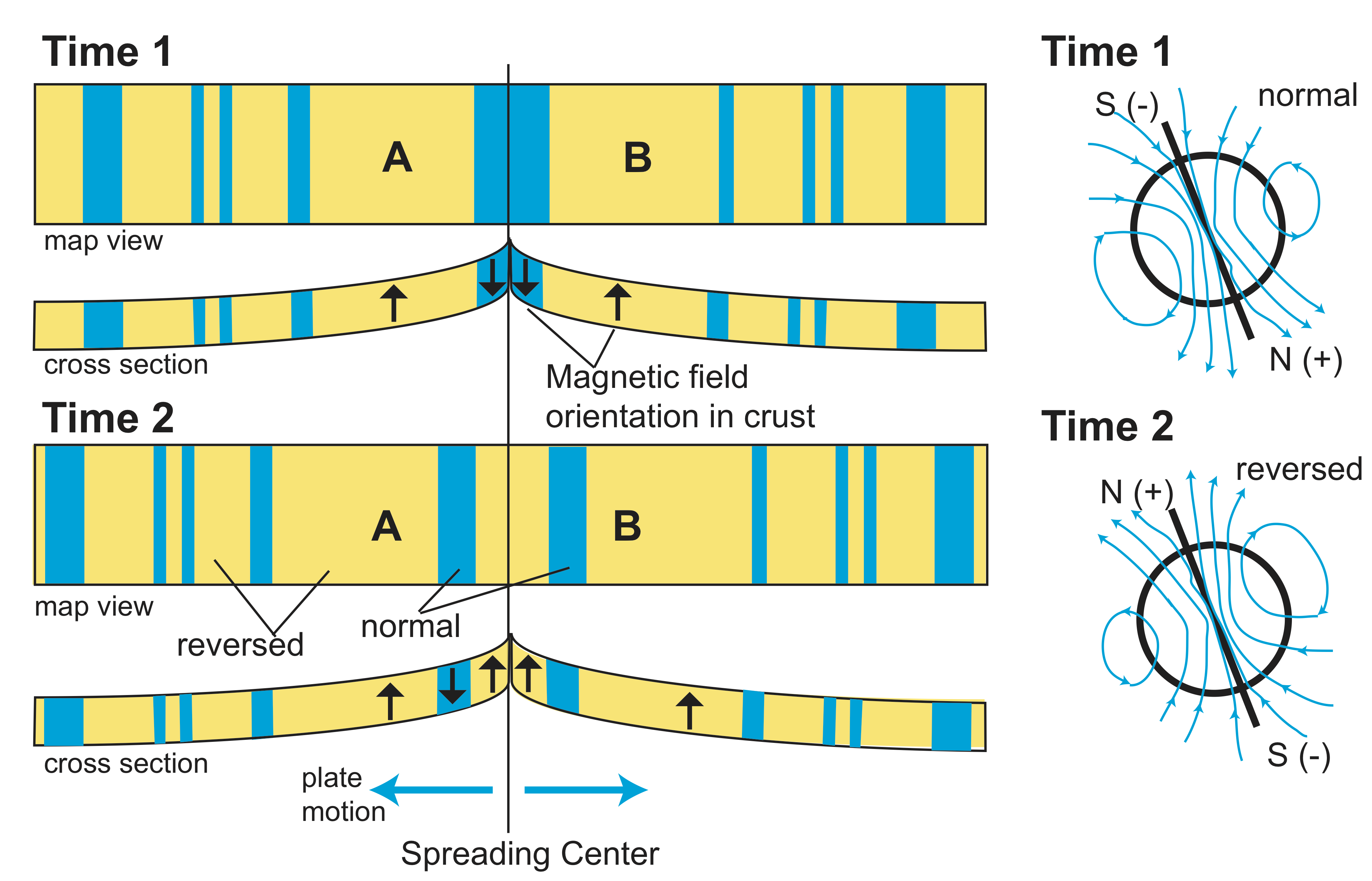
While there are multiple ways to determine the age of rocks, such as radiometric dating and fossil dating, for large-scale plate tectonic studies the most useful way of determining the age of plates is using magnetic stratigraphy. When sea floor is created at spreading centers magma is emplaced at shallow depth or erupted at the surface to form the crust of the growing plate. Certain minerals in the magma (e.g., magnetite) are sensitive to the Earth's magnetic field. As the magma cools, magnetic domains in these minerals will align with the Earth's magnetic field locking in the orientation (dip relative to horizontal) and polarity (field lines pointing out or field lines pointing in) of the magnetic field at that location. This would not be all that useful except that the Earth's magnetic field reverses direction in an aperiodic (non-repeating) pattern. Also, the Earth's magnetic field is dominated by a dipole field similar to what one gets from a simple bar magnet with a "north" end (positive end: magnetic field lines leave the magnet) and a "south" end (negative end: magnetic field lines enter the magnet). Therefore, at certain times the positive (north) pole of the magnetic field is close to the north pole of the Earth, while at other times the positive pole of the magnetic field is close to the south pole. Because this pattern of reversals is non-repeating, it acts like a bar code or finger print with a distinct pattern associated with different time intervals in the geologic past. At present, the negative magnetic pole located near the geographic north pole: this is termed a "normal" orientation. Times when the positive magnetic pole is located near the geographic north pole are termed "reversed".
Using lava eruptions on land, and dating these using radiometric dating methods, scientist have determined the pattern of reversals including the start and end times of each reversal going back about 250 million years. Using this "bar code" (called the Geomagnetic reversal time scale) one can determine the age of oceanic crust by measuring the present-day magnetic field, removing the contribution from the current magnetic field, and then analyzing the magnetic "anomalies" that remain. One must have some sense of whether the plate was in the northern or southern hemisphere at the time it formed. This is needed so we can determine whether a positive magnetic orientation is indicative of a "normal" orientation of the magnetic field or a reversal. The geographic orientation of the ridge can also cause the measured anomalies to appear asymmetric or skewed: this effect can be explored by calculating what anomalies would be expected for different orientations using calculation of the dipole field for the earth. Also, because the Earth's magnetic field is parallel to the Earth's surface at the magnetic equator, there is no information about the orientation of the magnetic field, and the crust in these locations can not be dated using magnetic stratigraphy.
Geomagnetic Timescale for the Neogene and Quaternary
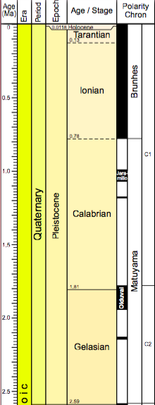
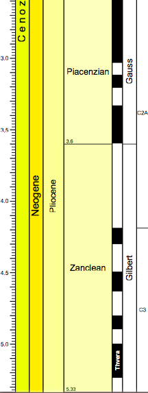
Figure \(\PageIndex{2}\): Neogene and Quaternary Timescale
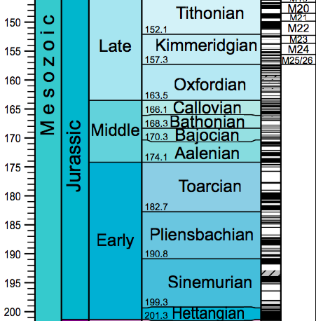
Geomagnetic Time-scale for 0 to 145 my
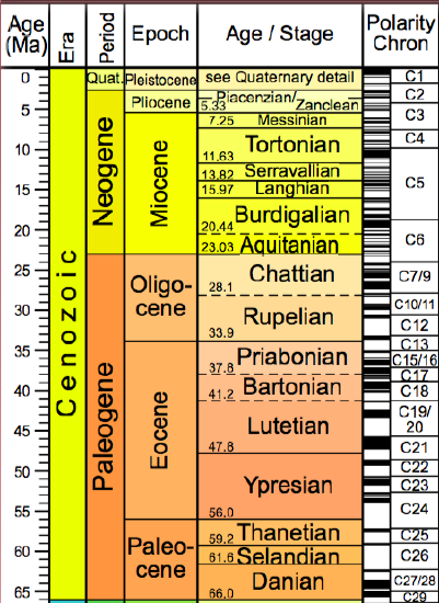
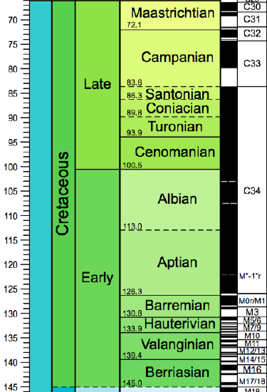
Figure \(\PageIndex{3}\): 0-145 My Geomagnetic Timescale
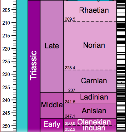
Geomagnetic Time-scale for 145 to 250 my
Take a little time to check out the patterns in the geomagnetic timescale shown above. What do you see? First note that when we just focus on the last 5 my, there are some very short reversals of the time-scale. Some are so short that they could be missed completely when looking at seafloor anomalies, especially at very slow spreading ridges in which time is represented by smaller widths of seafloor parallel to the spreading ridge. Second, notice the non-repeating nature of the pattern. There really is no pattern to speak of - this is exactly what makes it so useful for determining the age of seafloor. Third, notice that most of the periods of normal or reversed polarity at less than a million years to a few million years. There is one big exception to this and this is the very long period of normal polarity in Cretaceous, which extends from 126.3 to 83.6 my, a duration of 42.7 my. This long period of normal polarity is referred to as the Cretaceous quiet zone - quiet referring to the lack of magnetic field reversals.
Spreading Rate from Magnetic Anomalies
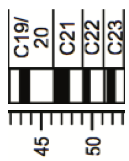
Determining the spreading rate (rate of crust accreted to the plate) from the magnetic anomalies is done in several steps. We assume that the magnetic anomalies have already been analyzed to identify the normal and reverse polarity anomalies taking into account the location (northern/southern hemisphere) and orientation (north-south versus east-west) of the ridge (north/south). You then have a "bar code" of normal and reverse polarity intervals of varying lengths. First, just look at the pattern (see example below) -- what do you see? Are there lots of reversals, or just a few. Are the reversals all similar length or different lengths? Is the pattern symmetric with respect to any point on the profile? This last question is key because a symmetric pattern indicates that there is an active or extinct spreading center in the profile, and therefore, you should only be considering the anomalies on one side of the profile in trying to match the pattern of reversals. Next, try to identify some specific pattern... short-short-long-long-short ... and find a similar pattern in the reference geomagnetic timescale. Here's a test section. Try finding where this fits in the time-scale above (hint its in the Cenozoic):

Note, you are looking at pattern, not the specific width of the reversals as these will depend on the actual spreading rate that formed the crust. A fast spreading rate will form wider bands because more crust is formed during each time interval. A slow spreading rate will form narrower bands. Initially, you should assume that the spreading rate was constant for the whole time interval. Once you think you have identify a section of the reference time-scale that matches your observation, look to the adjacent anomalies and see whether they also match with what comes next. If it matches - great, you can start marking down which normal and reverse isochrons match your profile. If they don't match, repeat the procedure until you find a consistent match of normal and reversed periods for the whole profile. Here's the solution to the above test section:
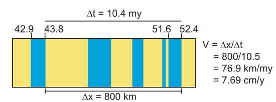
Once the anomalies are matched, the spreading rate is calculated by noting the start and end time of an anomaly at each end of the profile. Then calculate the time duration between the start or end of the first anomaly and the second anomaly \(\Delta t\) and the distance \(\Delta x\) between these two points on the profile. The spreading rate (velocity) is \( v_s = \frac{\Delta x}{\Delta t}\).
More Practice in Determining Spreading History
If we have time we can add this section with updated magnetic plots
This practice is very similar to what you will do in class.
For each profile:
- Determine if there is a pattern to the symmetry in the profile or not
- Look for distinct patterns that you can search for in the magnetic time-scale plots
- When you think you have a match, check that the adjacent patterns also fit
- Once you have a match, determine the age for the ends of the profile and symmetry position
- Determine the spreading history (the scale is in km)
- Describe in words a scenario for the history
FIGURE a
FIGURE f
FIGURE geomagnetic reversal time scale
FIGURE a answer
FIGURE f answer
10 my⇒\(\frac{100 km}{10 my}=100\frac{km}{my}\)
⇒Dead ridge:was spreading at ~\(\frac{100 mm}{10 yr}\) for 10 my then died at 155 my.