
4.1: The Forces Driving Plate Motions
- Page ID
- 3517

\( \newcommand{\vecs}[1]{\overset { \scriptstyle \rightharpoonup} {\mathbf{#1}} } \)
\( \newcommand{\vecd}[1]{\overset{-\!-\!\rightharpoonup}{\vphantom{a}\smash {#1}}} \)
\( \newcommand{\id}{\mathrm{id}}\) \( \newcommand{\Span}{\mathrm{span}}\)
( \newcommand{\kernel}{\mathrm{null}\,}\) \( \newcommand{\range}{\mathrm{range}\,}\)
\( \newcommand{\RealPart}{\mathrm{Re}}\) \( \newcommand{\ImaginaryPart}{\mathrm{Im}}\)
\( \newcommand{\Argument}{\mathrm{Arg}}\) \( \newcommand{\norm}[1]{\| #1 \|}\)
\( \newcommand{\inner}[2]{\langle #1, #2 \rangle}\)
\( \newcommand{\Span}{\mathrm{span}}\)
\( \newcommand{\id}{\mathrm{id}}\)
\( \newcommand{\Span}{\mathrm{span}}\)
\( \newcommand{\kernel}{\mathrm{null}\,}\)
\( \newcommand{\range}{\mathrm{range}\,}\)
\( \newcommand{\RealPart}{\mathrm{Re}}\)
\( \newcommand{\ImaginaryPart}{\mathrm{Im}}\)
\( \newcommand{\Argument}{\mathrm{Arg}}\)
\( \newcommand{\norm}[1]{\| #1 \|}\)
\( \newcommand{\inner}[2]{\langle #1, #2 \rangle}\)
\( \newcommand{\Span}{\mathrm{span}}\) \( \newcommand{\AA}{\unicode[.8,0]{x212B}}\)
\( \newcommand{\vectorA}[1]{\vec{#1}} % arrow\)
\( \newcommand{\vectorAt}[1]{\vec{\text{#1}}} % arrow\)
\( \newcommand{\vectorB}[1]{\overset { \scriptstyle \rightharpoonup} {\mathbf{#1}} } \)
\( \newcommand{\vectorC}[1]{\textbf{#1}} \)
\( \newcommand{\vectorD}[1]{\overrightarrow{#1}} \)
\( \newcommand{\vectorDt}[1]{\overrightarrow{\text{#1}}} \)
\( \newcommand{\vectE}[1]{\overset{-\!-\!\rightharpoonup}{\vphantom{a}\smash{\mathbf {#1}}}} \)
\( \newcommand{\vecs}[1]{\overset { \scriptstyle \rightharpoonup} {\mathbf{#1}} } \)
\( \newcommand{\vecd}[1]{\overset{-\!-\!\rightharpoonup}{\vphantom{a}\smash {#1}}} \)
\(\newcommand{\avec}{\mathbf a}\) \(\newcommand{\bvec}{\mathbf b}\) \(\newcommand{\cvec}{\mathbf c}\) \(\newcommand{\dvec}{\mathbf d}\) \(\newcommand{\dtil}{\widetilde{\mathbf d}}\) \(\newcommand{\evec}{\mathbf e}\) \(\newcommand{\fvec}{\mathbf f}\) \(\newcommand{\nvec}{\mathbf n}\) \(\newcommand{\pvec}{\mathbf p}\) \(\newcommand{\qvec}{\mathbf q}\) \(\newcommand{\svec}{\mathbf s}\) \(\newcommand{\tvec}{\mathbf t}\) \(\newcommand{\uvec}{\mathbf u}\) \(\newcommand{\vvec}{\mathbf v}\) \(\newcommand{\wvec}{\mathbf w}\) \(\newcommand{\xvec}{\mathbf x}\) \(\newcommand{\yvec}{\mathbf y}\) \(\newcommand{\zvec}{\mathbf z}\) \(\newcommand{\rvec}{\mathbf r}\) \(\newcommand{\mvec}{\mathbf m}\) \(\newcommand{\zerovec}{\mathbf 0}\) \(\newcommand{\onevec}{\mathbf 1}\) \(\newcommand{\real}{\mathbb R}\) \(\newcommand{\twovec}[2]{\left[\begin{array}{r}#1 \\ #2 \end{array}\right]}\) \(\newcommand{\ctwovec}[2]{\left[\begin{array}{c}#1 \\ #2 \end{array}\right]}\) \(\newcommand{\threevec}[3]{\left[\begin{array}{r}#1 \\ #2 \\ #3 \end{array}\right]}\) \(\newcommand{\cthreevec}[3]{\left[\begin{array}{c}#1 \\ #2 \\ #3 \end{array}\right]}\) \(\newcommand{\fourvec}[4]{\left[\begin{array}{r}#1 \\ #2 \\ #3 \\ #4 \end{array}\right]}\) \(\newcommand{\cfourvec}[4]{\left[\begin{array}{c}#1 \\ #2 \\ #3 \\ #4 \end{array}\right]}\) \(\newcommand{\fivevec}[5]{\left[\begin{array}{r}#1 \\ #2 \\ #3 \\ #4 \\ #5 \\ \end{array}\right]}\) \(\newcommand{\cfivevec}[5]{\left[\begin{array}{c}#1 \\ #2 \\ #3 \\ #4 \\ #5 \\ \end{array}\right]}\) \(\newcommand{\mattwo}[4]{\left[\begin{array}{rr}#1 \amp #2 \\ #3 \amp #4 \\ \end{array}\right]}\) \(\newcommand{\laspan}[1]{\text{Span}\{#1\}}\) \(\newcommand{\bcal}{\cal B}\) \(\newcommand{\ccal}{\cal C}\) \(\newcommand{\scal}{\cal S}\) \(\newcommand{\wcal}{\cal W}\) \(\newcommand{\ecal}{\cal E}\) \(\newcommand{\coords}[2]{\left\{#1\right\}_{#2}}\) \(\newcommand{\gray}[1]{\color{gray}{#1}}\) \(\newcommand{\lgray}[1]{\color{lightgray}{#1}}\) \(\newcommand{\rank}{\operatorname{rank}}\) \(\newcommand{\row}{\text{Row}}\) \(\newcommand{\col}{\text{Col}}\) \(\renewcommand{\row}{\text{Row}}\) \(\newcommand{\nul}{\text{Nul}}\) \(\newcommand{\var}{\text{Var}}\) \(\newcommand{\corr}{\text{corr}}\) \(\newcommand{\len}[1]{\left|#1\right|}\) \(\newcommand{\bbar}{\overline{\bvec}}\) \(\newcommand{\bhat}{\widehat{\bvec}}\) \(\newcommand{\bperp}{\bvec^\perp}\) \(\newcommand{\xhat}{\widehat{\xvec}}\) \(\newcommand{\vhat}{\widehat{\vvec}}\) \(\newcommand{\uhat}{\widehat{\uvec}}\) \(\newcommand{\what}{\widehat{\wvec}}\) \(\newcommand{\Sighat}{\widehat{\Sigma}}\) \(\newcommand{\lt}{<}\) \(\newcommand{\gt}{>}\) \(\newcommand{\amp}{&}\) \(\definecolor{fillinmathshade}{gray}{0.9}\)The motion of tectonic plates is driven by convection in the mantle. In simple terms, convection is the idea that dense, cold things sink, and buoyant, warm things rise. In the earth the cold sinking things are slabs (subducting plates) and the warm things are plumes, or just rising material from deeper in the mantle.
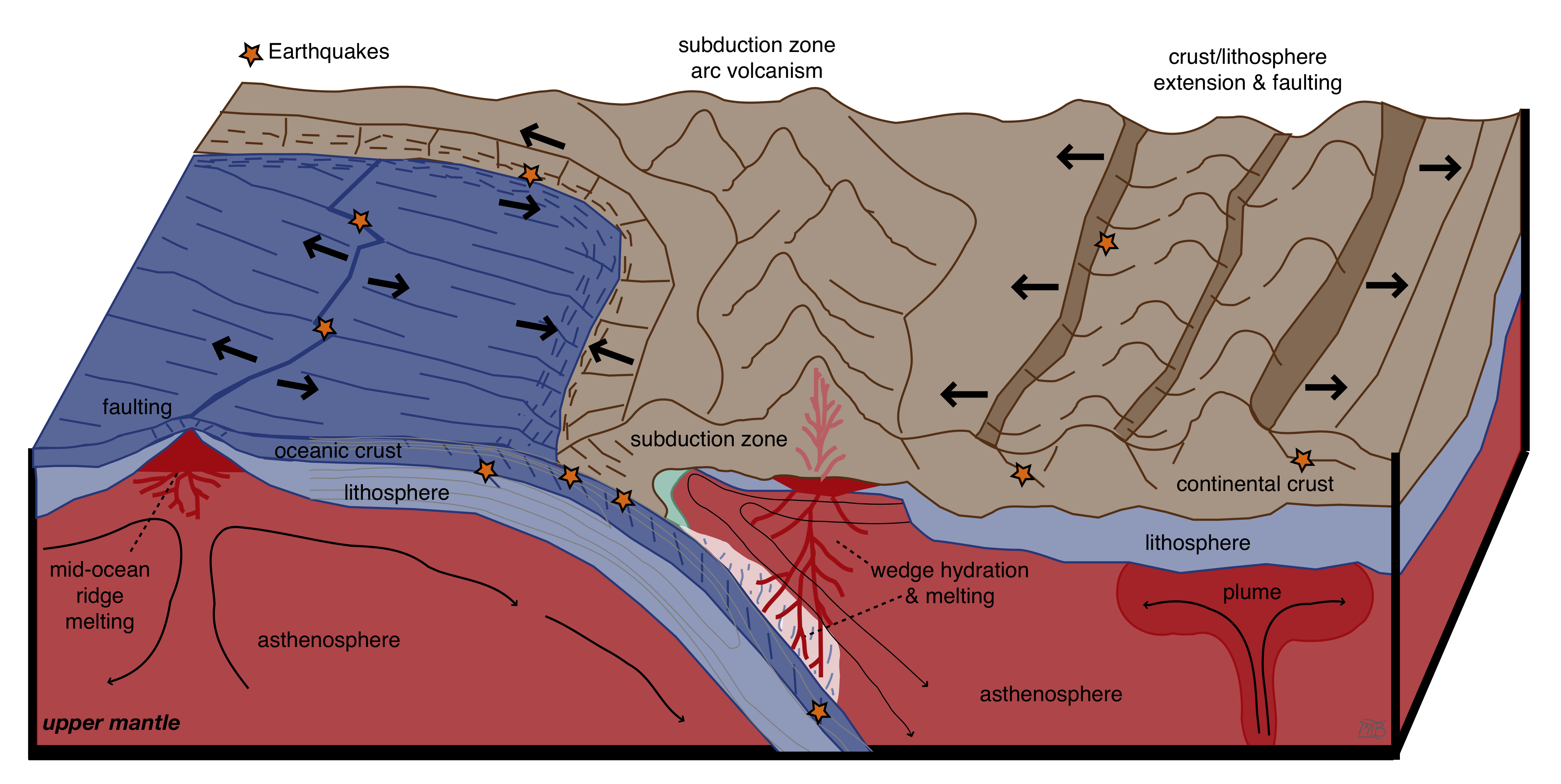
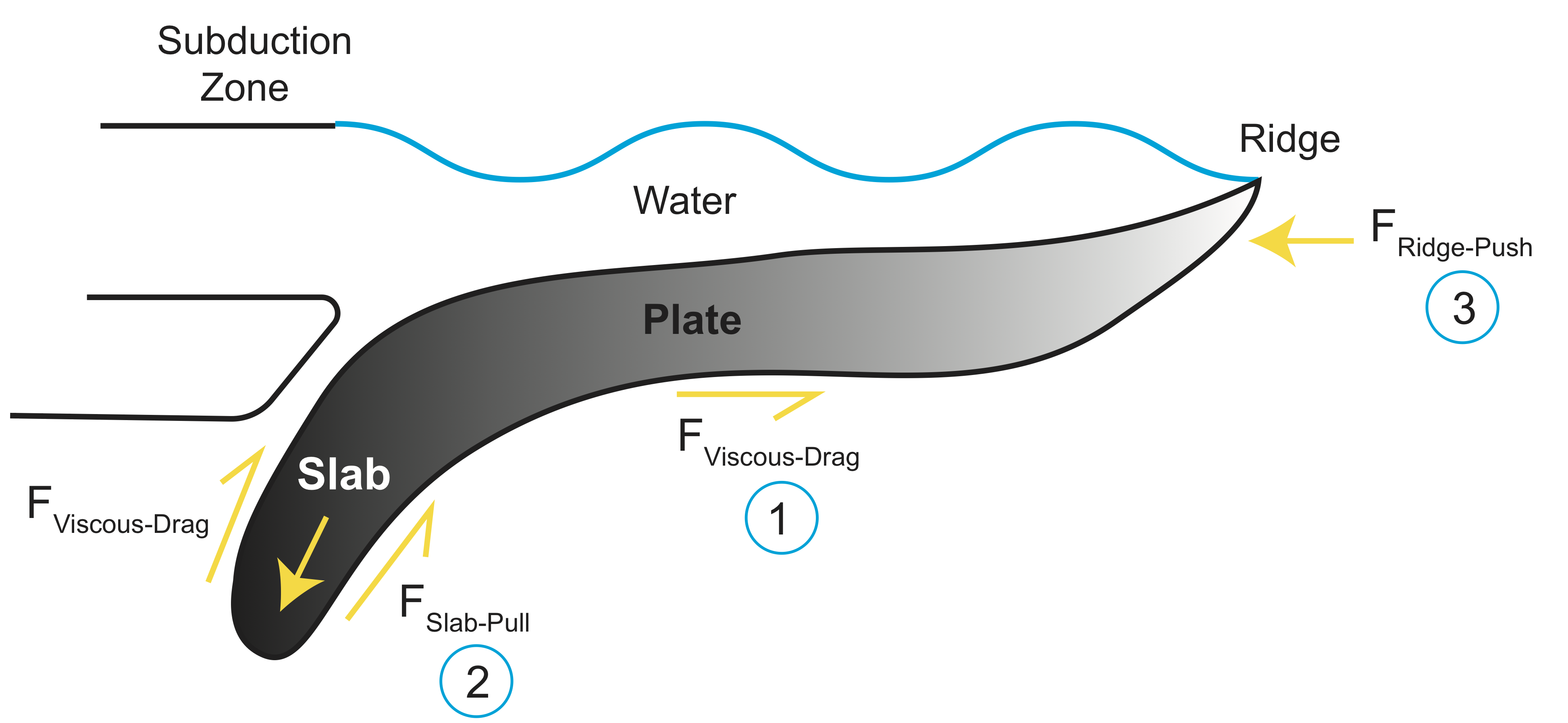
There are three main forces that determine the rate at which tectonic plates move as part of the mantle convection system:
- slab pull: the force due to the weight of the cold, dense sinking tectonic plate
- ridge push: the force due to the buoyancy of the hot mantle rising to the surface beneath the ridge.
- viscous drag: the force opposing motion of the plate and slab past the viscous mantle underneath or on the side.
This force balance is given by:
\[F_{ridge-push}+F_{slab-pull}-F_{viscous-drag}=0\]
Because the viscous drag depends explicitly on the plate velocity, it is possible to predict the speed plate motion when the forces are balanced (under certain simplifying assumptions).
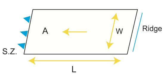
Recall from Chapter 1 that stress is related to force as \(\sigma=\frac{F}{A}\) where \(A = L W\). Rearranging, \(F=\sigma A\). When considering the force balance on the a plate it is useful to using a simplified geometry as shown below and consider the force per unit length (or ridge or subduction zone)
\[F= \sigma A/W = \sigma L \label{force}\]
As seen in the figure below, \(W\) is the length of the plate along the ridge and subduction zone. By considering the force per unit length (in the W direction), we can then consider the forces working along a profiles from the ridge to the subduction zone and ignore any variation in the ridge-parallel direction.
Viscous Drag
One of the mechanisms for plate motion that is a result of convection is viscous drag. This concept relates to ideas we discussed earlier, including the Couette Flow and viscous stress. The drag on the base of the oceanic lithosphere can both drive or resist plate motion, depending on the relative motion between the plate and the underlying mantle. For this discussion, we will consider that the plate is being pulled or pushed by slab-pull and ridge push and drags the asthenosphere with it. Therefore viscsous drag oppose the motion of the plate (or slab) and acts to slow it down.
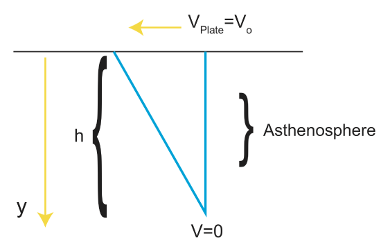
From the figure above, we can derive an equation to describe plate motion due to viscous drag.
\[V=V_o(1-\frac{y}{h})\]
\[\dot{\varepsilon}=\frac{1}{2}\frac{dV}{dy}=-\frac{V_o}{2h}\]
\[\begin{align*}\sigma &=2\eta\dot{\varepsilon} \\[4pt] &=2\eta(\frac{-V_o}{2h}) \\[4pt] &=\frac{-V_o\eta}{h} \end{align*}\]
The negative sign indicates an opposition to plate motion, i.e., the viscous drag. We now have an equation that describes the magnitude of drag:
\[|\sigma|=\frac{V_o\eta}{h}\]
placing this into our previous force equation (Equation \ref{force}):
\[F=\sigma L = \frac{V_o\eta}{h} L\]
Let's do an example calculating viscous drag under a plate.
Example Viscous Drag Under the Plate
Assume that:
- the plate drags the mantle underneath in a layer that is 100 km thick (h~100 km).
- the mantle viscosity is \(\eta ~ 1\times10^{18}\) Pa(s).
- the plate velocity is Vo~5 cm/yr. (Note that this is equivalent to 0.05 m/yr = 50 mm/yr = 50 km/my
- the plate length from the ridge to the subduction zone is about 5000 km
From the strain-rate, we can get the stress as shown above, and then multiply by the length of the plate
Using these numbers, we can calculate the force on the descending plate, \(F=1.59 \times 10^{11}\) N/m.
The above example is for the viscous drag just under the plate, but now we will also consider a case where there are stresses acting on both sides of the subducting slab. As the slab sinks into the mantle, the viscous mantle on both sides resists the sinking motion of the slab. For this simple example,
\[\sigma=\frac{V_o\eta_{av}}{h}\]
\[F=\sigma L_{slab}\]
\[F_{vis.}=2F=2\sigma L_{slab}=\frac{2V_o\eta_{av}}{h}L_{slab}\]
Example Viscous Drag on Two Sides of a Plate
As we did in the previous example, consider viscous drag on a slab, but now on both sides of the plate.
We are given that
- The slab sinks at the same speed that the plate is moving: Vo=Vplate~5 \(\frac{cm}{yr}\),
- Again, the shearing layer on both sides is 100 km wide (h~100 km),
- The viscosity of the mantle increases with depth, for this example we'll assume its constant \(\eta_{av} =10^{21}\) Pa s ,
- The slab length (from the base of the lithosphere to the upper/lower mantle boundary is Lslab = 560 m.
In this case, \(F = 78 \times 10^{13}\) N/m. If we change \(\eta\) to \(10^{21}\), then equals \(F=1.78x10^{10}\) N/m.
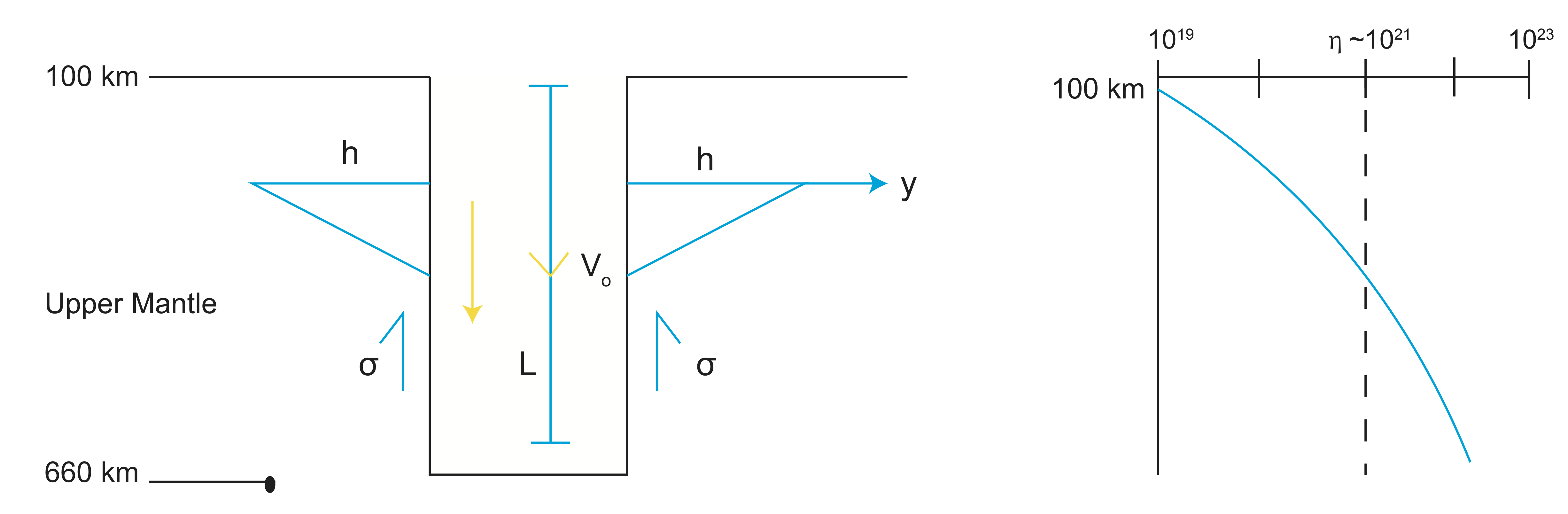
Figure \(\PageIndex{5}\): Force on a Descending Plate
On the sides of the slab, the above figures demonstrate the forces that are present. We can also see that the slab is sinking vertically, which is not often the case in the real world. From the right figure, \(\eta\approx 10^{21}\). This is actually too high because of non linear viscosity, but we are ignoring other things so it works for this example.
Notice that the stress is proportional to the velocity \(\sigma \alpha V\) so as the velocity increases so does the stress opposing the sinking.
However, the biggest changes come from the viscosity because it can changes by x10-100 in the upper mantle, thus this change has the biggest effect on the viscous drag.
The viscous drag is also proportional to the length of the slab, so the resistance also increases as the slab gets longer (but so does the slab pull force).
Slab-Pull Force
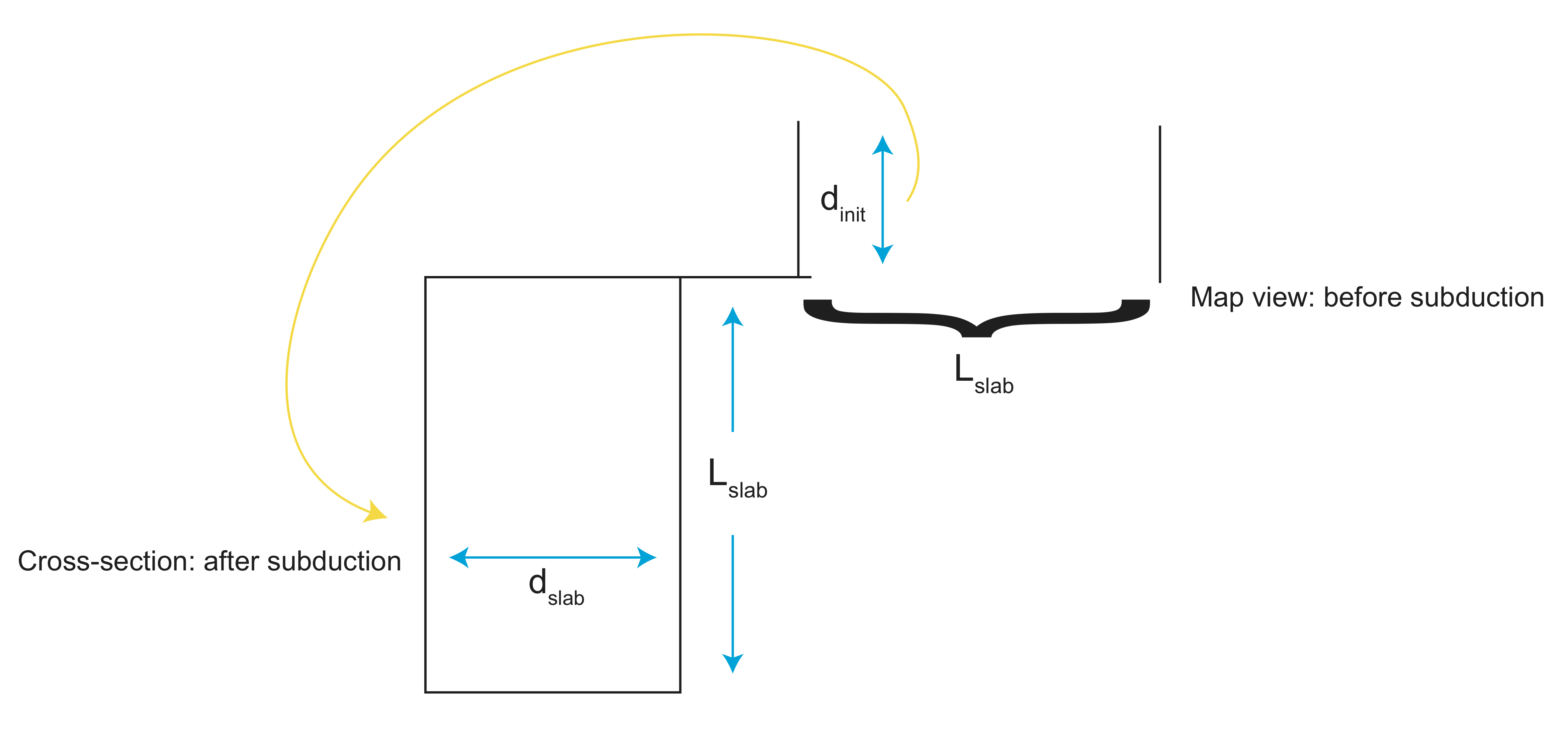
The main force on a subducting plate is the slab-pull force. This is the force due to the density contrast between a slab and its surroundings, ie., the mass anomaly of the slab in the mantle. We can approximate this force by thinking of the sinking slab a a vertical rectangle (like the viscous drag example) with a width, \(w\), hanging down a distance, \(d\) from the Earth's surface with a temperature \(\Delta T\) different than its surroundings.
The density as a function of temperature is given by
\[\rho (T)=\rho_m(1+\alpha (T_m - T))\]
where \(\rho_m \) is the reference mantle density at \(T = T_m\) and cold material has a higher density, and \(\alpha\) is the thermal expansion coefficient and is ~\(2 \times 10^{-5}\) 1/K in the sinking slab.
For the slab, we can rewrite this as:
\[\rho (T)=\rho_m(1+\alpha \Delta T)\]
where \(\Delta T=T_m-T_{slab}\)
The density anomaly is then
\[\Delta \rho= \rho_m\alpha\Delta T\]
This is the extra density of the slab relative to the mantle. To calculate the force per unit area, we need to determine the mass anomaly per unit area, \(\Delta M = \Delta \rho A_{slab} \), where A_{slab} is the cross sectional area of the slab along the profile (width across times length into the mantle).
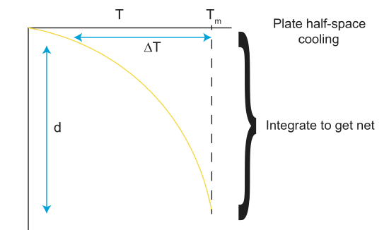
The temperature in the slab is related to the temperature of the subducting plate. Recall from the chapter on thermal diffusion that the temperature of a tectonic plate is given by the half-space cooling model. Once the plate starts sinking, the cold slab warms up, and the surrounding mantle cools down. However, the total temperature anomaly (temperature difference times volumes) stays the same. (Remember that there is conservation of energy, so the total energy of the cold slab is conserved). So, if we integrate the temperature profile solution from the half-space cooling model over the thickness of this plate, this will also be the thermal anomaly of the the slab. Finally, because the density anomaly is just \[\Delta \rho=\rho_m\alpha\Delta T\], we can get the total density anomaly by just multiplying by \(\rho_m \alpha\).
So, the trick to figuring out the slab pull force is the first determine the density anomaly of the subducting plate just before it enters the trench. Then imagine taking a length of plate equal to the length of the slab and rotating it en masse in to the mantle. The density anomaly of the sinking slab will be the same.
To get the density anomaly, we integrate the temperature equation for the plate from the half-space cooling model.
\[T(z, t)=(T_s-T_m)erfc(\frac{z}{2\sqrt{\kappa t}})+T_m\]
Here \(z\) is the depth through the subducting plate, before it sinks, or the width through the slab while it is sinking.
\[\Delta T=T_m - T(z, t)\]
\[\Delta T=-(T_s-T_m)erfc(\frac{z}{2\sqrt{\kappa t}})\]
\[\Delta T=(T_s-T_m)erfc(\frac{z}{2\sqrt{\kappa t}})\]
Then, multiplying the \(\rho_m \alpha\),
\[\Delta \rho=\rho_m\alpha\Delta T\]
\[\Delta \rho=\rho_m\alpha\Delta T(z)\]
Next we integrate over the width (depth) to the get the mass per unit length (length parallel to the trench) in a single profile, (we will need to sum this over the length of the slab):
\[\Delta m=\int_{0}^{z\rightarrow\infty}{\Delta \rho(z)dz}\]
\[\Delta m=\rho_m\alpha(T_m-T_s)\int_{0}^{\infty}erfc(\frac{z}{2\sqrt{\kappa t}})dz\]
Now we use variable substitution so we can solve the integral
Let \(q=\frac{z}{2\sqrt{\kappa t}}\) where \(z\rightarrow\infty\) and \(q\rightarrow\infty\).
\[\frac{dq}{dz}=\frac{1}{2\sqrt{\kappa t}}\]
\[dz=2\sqrt{\kappa t}dq\]
Now substitute into the integral,
\[\Delta m=\rho_m\alpha(T_m-T_s)2\sqrt{\kappa t}\int_{0}^{\infty}erfc(q)dq\]
The complementary error function integral solution can be found in any integral table (or search online) and equals \(\sqrt{\frac{1}{\pi}}\)
\[\Delta m=\rho_m\alpha(T_m-T_s)2\sqrt{\frac{\kappa t}{\pi}}\]
The above equation gives the mass anomaly (relative to the surrounding mantle) per unit length.
Finally, we can determine the total mass anomaly by multiplying by the length of the slab:
\[\Delta M=\Delta m L_{slab}\]
The slab pull force is then given by,
\[F_{slab-pull}=\Delta m L_{slab} g\]
and subsituting for \(\Delta m\),
\[F_{sp}=2 \rho_m\alpha (T_m-T_s) g L_{slab}\sqrt{\frac{\kappa t}{\pi} } \]
Example Slab-Pull Force
We are given that
- \(\rho_o\)=3300 kg/m\(^3\),
- \(\alpha =2e-5\) 1/K, g=9.81 m/s\(^2\),
- Tm-Ts=1400 K,
- \(\kappa =1e-6\) m\(^2\)/s,
- t=age of slab at time of subduction,
- Lslab=560 km.
We know that \(F_{sp}=\Delta m L_{slab} g\)
Thus, the force per unit length of the slab-pull is Fsp=2.88x10¹³ N/m
You might notice that this force is 100 - 1000x more than the viscous drag force.
Ridge-Push Force
Let's cover a final force a subducting plate would experience, the ridge-push force. This force results from the elevation of oceanic ridges above the seafloor. This difference in height leads to pressure that 'pushes' the plate away from the ridge. Ridge push is the simplest force in some ways, as all its components can be easily examined.

Simply put, to determine ridge-push forces, we need to do two things. First, look at the isostatic balance and the depth of oceans w(t). Second, we need to look at the force balance on the plate.
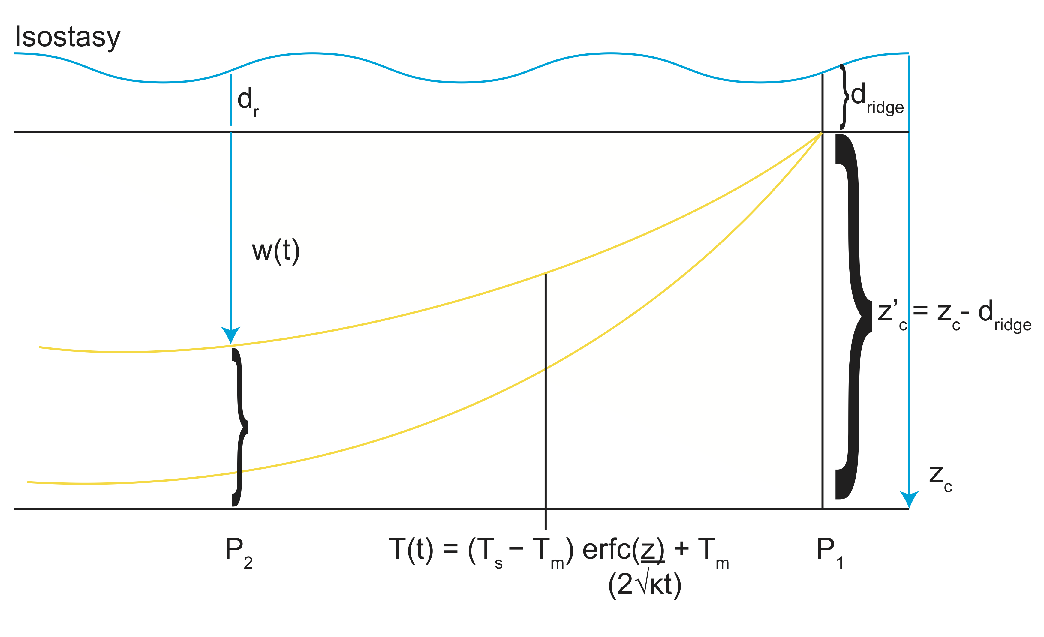
\[T(t)=(T_s-T_m)erfc(\frac{z}{2\sqrt{\kappa t}})+T_m\]
\[\rho(T)=\rho_m(1+\alpha\Delta T)\]
\[\Delta T=T_m-T(t)\]
T(t) is <Tm+\(\Delta T\) because of more density.
Balance pressures:
P1=P2
\[drp_wg+\int_{dr}^{dr+w}\rho (T)gdz+\int_{dr+w}^{z_c}\rho (T)gdz=(dr+w)\rho_wg + \int_{dr+w}^{z_c}\rho (T)gdz\]
\[\int_{dr}^{dr+w}\rho_mdz+\int_{dr+w}^{z_c}\rho_mdz=wp_w+\int_{dr+w}^{z_c}\rho (z)dz\]
\[w\rho_m-wp_w=\int_{dr+w}^{z_c}\rho (z)-\rho_mdz\]
\[\rho (z)=\rho (T)\rightarrow T(z)\]
Like we did above, we will use the complementary error function and find its solution in a integral table.
\[w(\rho_m-\rho_w)=\rho_m\alpha(T_m-T_s)\int_{0}^{\infty}erfc(\frac{z'}{2\sqrt{\kappa t}})dz'\]
The complementary error function integral solution is \(2\sqrt{\frac{\kappa t}{\pi}}\)
\[w=\frac{2\rho_m\alpha(T_m-T_o)}{\rho_m-\rho_w}\sqrt{\frac{\kappa t}{\pi}}\]
An important thing to note is that the depth of the ocean basins deepen at ~\(\sqrt{t}\) (the square root of age)
⇒balanced pressures (isostasy)
Ridge-push is very similar to the balanced pressures idea, but uses balanced forces instead.
⇒\(\Delta P\)⇒drives flow across A. No net force⇒no \(\Delta P\).
\[F\backsim\Delta P A\] This is the force per unit width.
Example Ridge-Push
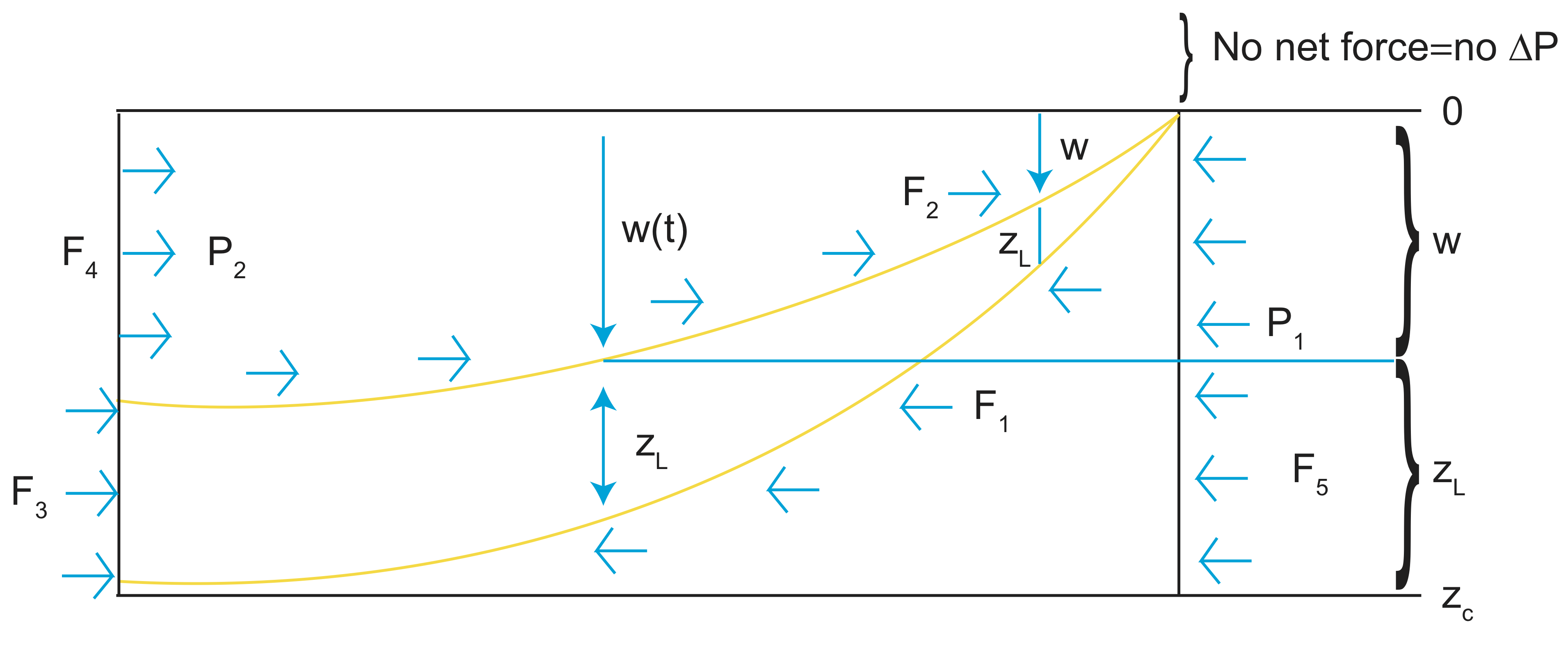
The forces in this example should balance. After we write the integrals for the various forces, we should have an expression where FRP=F1-F2-F3.
\[F_1=\int_{0}^{z_c}\rho_mgzdz=F_s\]
Here, \(\rho_mgz\) represents the pressure, dz is XA⇒Area⇒wXL\(\frac{area}{w}\)=L
We can do a simple integral in depth, this is the same pressure from the mantle below a plate.
Rewriting F1 0→zc, 0→w + w-zL
\[F_1=\int_{0}^{w}\rho_mgzdz+\int_{w}^{w+z_c}\rho_mgzdz+\int_{0}^{2L}\rho_mg\bar{z}d\bar{z}\]
Where we let \(\bar{z}=z-w\)
\[F_2=\int_o^w\rho_wgz=F_4\]
\(\rho_wgz\) is P2. Here, we do not need to integrate over shape of w.
\[F_3=\int_0^{z_L}P_Ld\bar{z}\]
\[P_L=\rho_w g w+\int_0^{\bar{z}} \rho_L (T)g d\bar{z}\]
Here, \(\rho_w g w\) is the pressure due to the water and \(\rho_L\) is the temperature-dependent density of the lithosphere.
Remember our force balance equation:
\[ F_{RP}=F_1-F_2-F_3\]
Plugging everything in and skipping some of the basic algebra we get:
\[F_{RP}=g[\frac{1}{2}(\rho_m-\rho_w)w^2+\kappa t\rho_m\alpha(T_m+T_s)]\]
We get the term w2 because PL~w and we integrated PL.
From isostasy, we can plug in
\[w(t)=\frac{2\rho_m\alpha(T_m-T_s)}{(\rho_m-\rho_w)}\sqrt{\frac{\kappa t}{\pi}}\]
\[F_{RP}=g \rho_m\alpha(T_m-T_s) \kappa t (1+\frac{2p_m\alpha(T_m-T_s)}{\pi(\rho_m-\rho_w)})\]
Notes on Ridge-Push
A few things to note: isostasy→controlling w(t)
The pressure across the lithosphere→ridge-push force
FRP\(\alpha\)t age of the oldest part of plate
Now that we have our general solution for the ridge-push force, if we are given actual values, we can solve it. If g=9.81, k=1e-6\(\frac{m^2}{s}\), \(\rho_m\)=3300\(\frac{ky}{m^3}\), Tm-Ts=1400 K, \(\alpha\)=2x10⁻⁵\(\frac{1}{K}\), \(\rho_m\)=1000\(\frac{kg}{m^3}\), we can finally find the force
\[F_{RP}=3.24x10^{12}\frac{N}{m}\]