3.5: Observing the Gravity Field
- Page ID
- 3523

\( \newcommand{\vecs}[1]{\overset { \scriptstyle \rightharpoonup} {\mathbf{#1}} } \)
\( \newcommand{\vecd}[1]{\overset{-\!-\!\rightharpoonup}{\vphantom{a}\smash {#1}}} \)
\( \newcommand{\id}{\mathrm{id}}\) \( \newcommand{\Span}{\mathrm{span}}\)
( \newcommand{\kernel}{\mathrm{null}\,}\) \( \newcommand{\range}{\mathrm{range}\,}\)
\( \newcommand{\RealPart}{\mathrm{Re}}\) \( \newcommand{\ImaginaryPart}{\mathrm{Im}}\)
\( \newcommand{\Argument}{\mathrm{Arg}}\) \( \newcommand{\norm}[1]{\| #1 \|}\)
\( \newcommand{\inner}[2]{\langle #1, #2 \rangle}\)
\( \newcommand{\Span}{\mathrm{span}}\)
\( \newcommand{\id}{\mathrm{id}}\)
\( \newcommand{\Span}{\mathrm{span}}\)
\( \newcommand{\kernel}{\mathrm{null}\,}\)
\( \newcommand{\range}{\mathrm{range}\,}\)
\( \newcommand{\RealPart}{\mathrm{Re}}\)
\( \newcommand{\ImaginaryPart}{\mathrm{Im}}\)
\( \newcommand{\Argument}{\mathrm{Arg}}\)
\( \newcommand{\norm}[1]{\| #1 \|}\)
\( \newcommand{\inner}[2]{\langle #1, #2 \rangle}\)
\( \newcommand{\Span}{\mathrm{span}}\) \( \newcommand{\AA}{\unicode[.8,0]{x212B}}\)
\( \newcommand{\vectorA}[1]{\vec{#1}} % arrow\)
\( \newcommand{\vectorAt}[1]{\vec{\text{#1}}} % arrow\)
\( \newcommand{\vectorB}[1]{\overset { \scriptstyle \rightharpoonup} {\mathbf{#1}} } \)
\( \newcommand{\vectorC}[1]{\textbf{#1}} \)
\( \newcommand{\vectorD}[1]{\overrightarrow{#1}} \)
\( \newcommand{\vectorDt}[1]{\overrightarrow{\text{#1}}} \)
\( \newcommand{\vectE}[1]{\overset{-\!-\!\rightharpoonup}{\vphantom{a}\smash{\mathbf {#1}}}} \)
\( \newcommand{\vecs}[1]{\overset { \scriptstyle \rightharpoonup} {\mathbf{#1}} } \)
\( \newcommand{\vecd}[1]{\overset{-\!-\!\rightharpoonup}{\vphantom{a}\smash {#1}}} \)
\(\newcommand{\avec}{\mathbf a}\) \(\newcommand{\bvec}{\mathbf b}\) \(\newcommand{\cvec}{\mathbf c}\) \(\newcommand{\dvec}{\mathbf d}\) \(\newcommand{\dtil}{\widetilde{\mathbf d}}\) \(\newcommand{\evec}{\mathbf e}\) \(\newcommand{\fvec}{\mathbf f}\) \(\newcommand{\nvec}{\mathbf n}\) \(\newcommand{\pvec}{\mathbf p}\) \(\newcommand{\qvec}{\mathbf q}\) \(\newcommand{\svec}{\mathbf s}\) \(\newcommand{\tvec}{\mathbf t}\) \(\newcommand{\uvec}{\mathbf u}\) \(\newcommand{\vvec}{\mathbf v}\) \(\newcommand{\wvec}{\mathbf w}\) \(\newcommand{\xvec}{\mathbf x}\) \(\newcommand{\yvec}{\mathbf y}\) \(\newcommand{\zvec}{\mathbf z}\) \(\newcommand{\rvec}{\mathbf r}\) \(\newcommand{\mvec}{\mathbf m}\) \(\newcommand{\zerovec}{\mathbf 0}\) \(\newcommand{\onevec}{\mathbf 1}\) \(\newcommand{\real}{\mathbb R}\) \(\newcommand{\twovec}[2]{\left[\begin{array}{r}#1 \\ #2 \end{array}\right]}\) \(\newcommand{\ctwovec}[2]{\left[\begin{array}{c}#1 \\ #2 \end{array}\right]}\) \(\newcommand{\threevec}[3]{\left[\begin{array}{r}#1 \\ #2 \\ #3 \end{array}\right]}\) \(\newcommand{\cthreevec}[3]{\left[\begin{array}{c}#1 \\ #2 \\ #3 \end{array}\right]}\) \(\newcommand{\fourvec}[4]{\left[\begin{array}{r}#1 \\ #2 \\ #3 \\ #4 \end{array}\right]}\) \(\newcommand{\cfourvec}[4]{\left[\begin{array}{c}#1 \\ #2 \\ #3 \\ #4 \end{array}\right]}\) \(\newcommand{\fivevec}[5]{\left[\begin{array}{r}#1 \\ #2 \\ #3 \\ #4 \\ #5 \\ \end{array}\right]}\) \(\newcommand{\cfivevec}[5]{\left[\begin{array}{c}#1 \\ #2 \\ #3 \\ #4 \\ #5 \\ \end{array}\right]}\) \(\newcommand{\mattwo}[4]{\left[\begin{array}{rr}#1 \amp #2 \\ #3 \amp #4 \\ \end{array}\right]}\) \(\newcommand{\laspan}[1]{\text{Span}\{#1\}}\) \(\newcommand{\bcal}{\cal B}\) \(\newcommand{\ccal}{\cal C}\) \(\newcommand{\scal}{\cal S}\) \(\newcommand{\wcal}{\cal W}\) \(\newcommand{\ecal}{\cal E}\) \(\newcommand{\coords}[2]{\left\{#1\right\}_{#2}}\) \(\newcommand{\gray}[1]{\color{gray}{#1}}\) \(\newcommand{\lgray}[1]{\color{lightgray}{#1}}\) \(\newcommand{\rank}{\operatorname{rank}}\) \(\newcommand{\row}{\text{Row}}\) \(\newcommand{\col}{\text{Col}}\) \(\renewcommand{\row}{\text{Row}}\) \(\newcommand{\nul}{\text{Nul}}\) \(\newcommand{\var}{\text{Var}}\) \(\newcommand{\corr}{\text{corr}}\) \(\newcommand{\len}[1]{\left|#1\right|}\) \(\newcommand{\bbar}{\overline{\bvec}}\) \(\newcommand{\bhat}{\widehat{\bvec}}\) \(\newcommand{\bperp}{\bvec^\perp}\) \(\newcommand{\xhat}{\widehat{\xvec}}\) \(\newcommand{\vhat}{\widehat{\vvec}}\) \(\newcommand{\uhat}{\widehat{\uvec}}\) \(\newcommand{\what}{\widehat{\wvec}}\) \(\newcommand{\Sighat}{\widehat{\Sigma}}\) \(\newcommand{\lt}{<}\) \(\newcommand{\gt}{>}\) \(\newcommand{\amp}{&}\) \(\definecolor{fillinmathshade}{gray}{0.9}\)Observing (Measuring) the Gravity Field on Earth
The gravity field of the Earth is determined in two ways:
- Measuring the orbits of satellites and using these to determine the gravity field. Early on this was done with single satellites and this provided the long wavelength observation of the gravity field (able to capture features down to about 100 km by the year 2000). Now these observations are done with twin satellites that orbit in tandem known as the GRACE mission (ADD LINK). Because satellites are not at the Earth's surface but rather are thousands of kilometers above the Earth's surface and gravity decreases with distances, these measurements always provide a smoother picture of gravity than what actually exists at the surface.
- Because 70% of the earth's surface is covered in water, a higher resolution observations of the gravity field can be measured by measuring the height of the ocean surface. This is done using a technique called satellite radar altimetery [ADD LINK] in which the distance between a satellite and the sea surface is measured. Repeated measurements removes the signal due to waves and currents (this signal is used by oceanographers to map where the currents are flowing).
Satellite altimetry provides a very high resolution image of the gravity field. This measurement is so high resolution that it can be converted into a map of seafloor topography and used to locate plate boundaries, fracture zones and seamounts both big and small. It is not high resolution enough to use for navigation of a real boat. However, if you use google maps and turn topography on, and got hunting around off the coast, the background topography images for the globe is the topography derived from satellite altimetry. If you zoom in really close near a port, you will see that there are regions with much finer resolution, this is because there is shipboard mapping of the seafloor that is "stitched" onto the background image.
Geoid Height from Satellite Altimetry
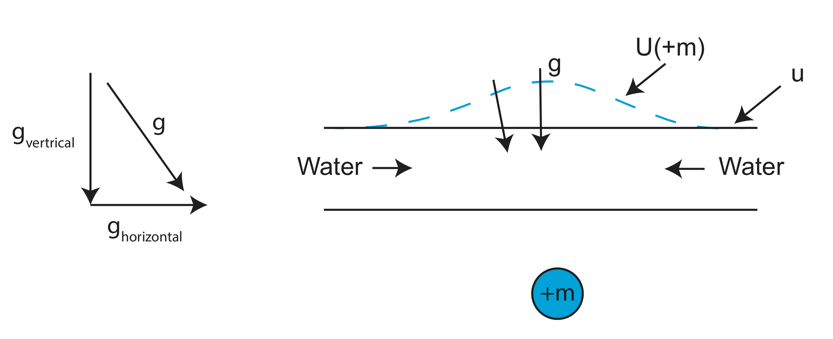
Some things to note about and what influences it:
- There is a layer of water→ocean
- U is parallel to surface, g is perpendicular
- Add a mass anomaly
- U moves out
- g is deflected→ it now has a horizontal component
- Water flows in created a bump
- Now the sea surface follows Uobs
Satellite altimetry is measuring the geoid. Gravity (g) is then calculated from the geoid by taking the spatial derivative.
Because the sea surface follows the geoid, we can visualize the geoid height as that height of the ocean surface above or below a reference surface. Note that the fact that water surface follows the geoid means means that sea-level is not at the same height (relative to the center of the Earth) everywhere.
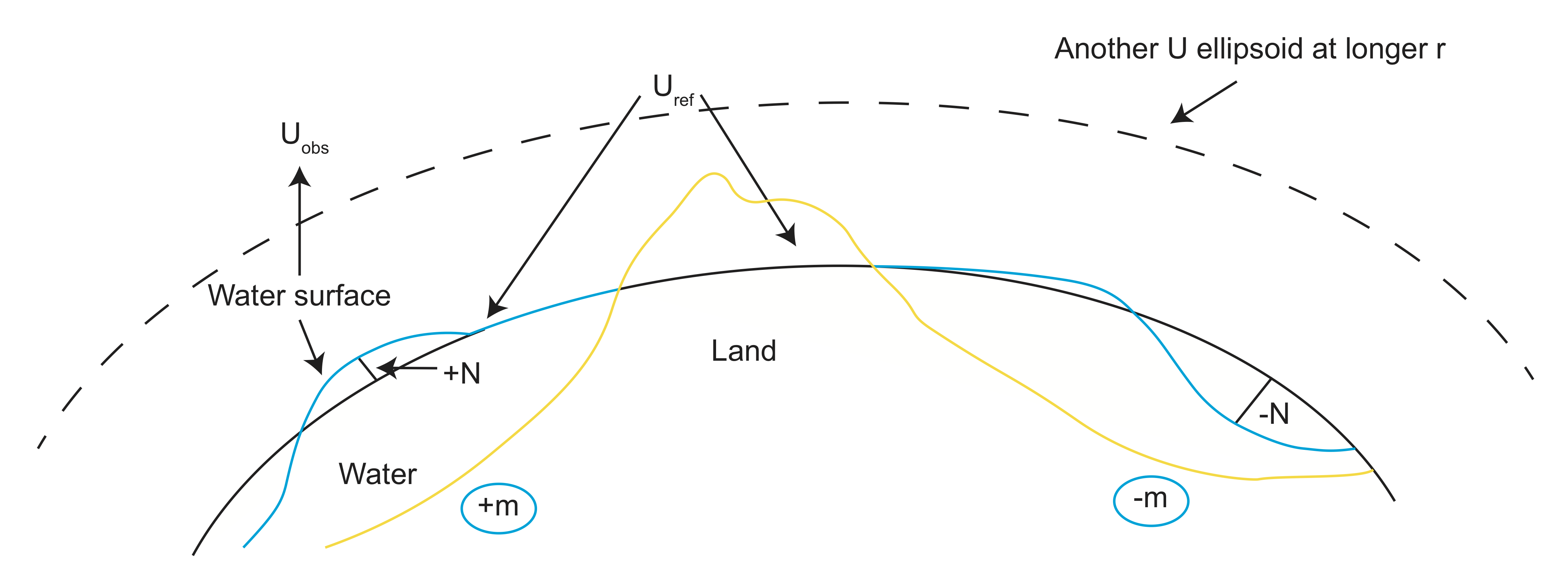
- Land and water
- Uref→cuts through these
- Uobs→undulations due to mass
- Uobs-Uref→geoid height→N
+N over +m and -N over -m. |N|→\(\pm\)100 meters
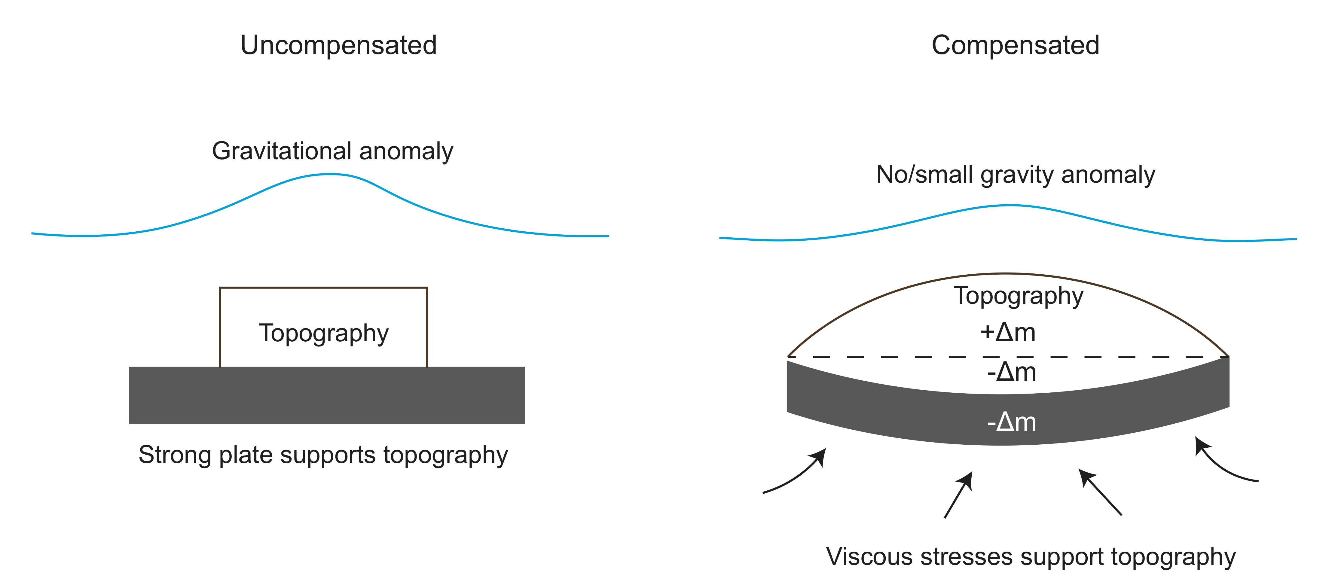
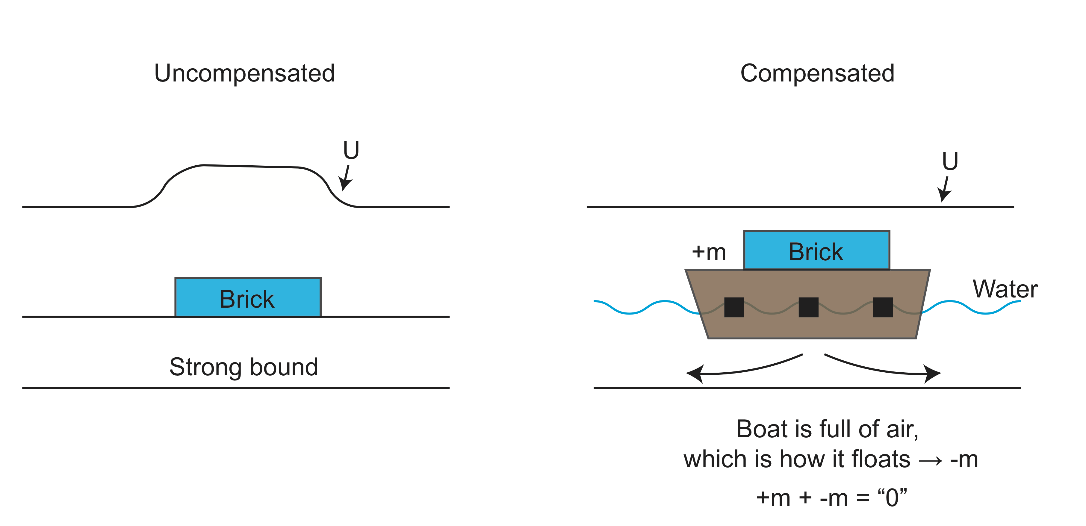
Compensated and Uncompensated Topography [need to move to its own section]
Topography at the Earth's surface is not always visible through the gravity field. For example, there is not an offset in gravity associated with going from the oceans to the continents despite the fact that the continents sit several kilometers higher. For some topography the positive mass anomaly of the topography is balanced (compensated) by a negative mass anomaly due to thicker crust. This is the case the continents. The continents are higher because the continental crust is thicker and lower density than the crust of the oceanic regions. Only uncompensated topography will have a signal in the gravity field. Some mass anomalies can also be "partially" compensated, so that the gravity signal is less than expected based on the topography.
The figure below illustrates the concepts of uncompensated and compensated topography. On the left imagine a brick on a stiff board that doesn't bend. This brick is an uncompensated mass on top of the board. It will have a signal in the gravity field. On the right imagine putting that brick on a small boat filled with air. The boat is pushed into the water by the weight of the brick until the weight is balanced (compensated). In this case there is not gravity signal because the anomaly from the brick is cancelled out by the anomaly of the submerged portion of the boat.
We will return to this concept in the discussion of isostasy [ADD LINK].
Smaller features
- seamounts
- fracture zones
- trenches
- These are all compensated and supported by the strength of the lithosphere
- ⇒gravity anomaly
Bigger features
- continents
- mountain ranges
- compensated or "floating"
- Uncompensated and supported by viscous stresses, often mantle has flowed away⇒isotasy
- ⇒no gravity anomaly
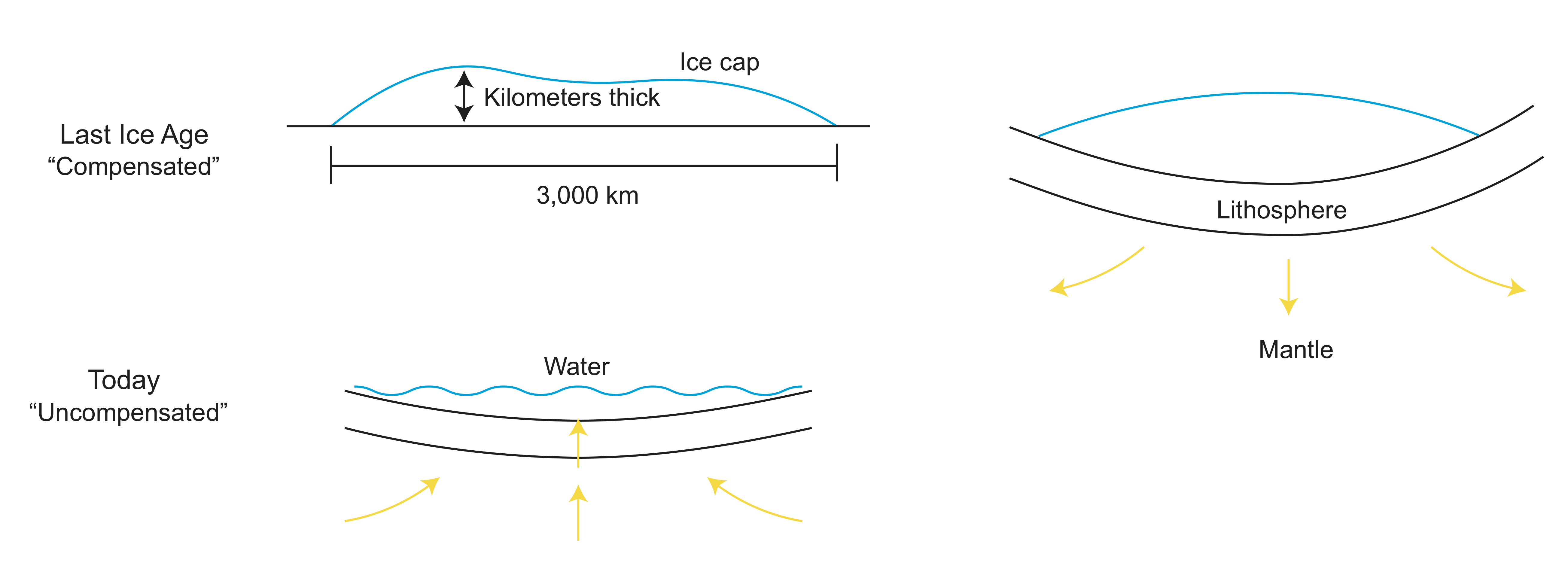
Hudson Bay
Let's look at an example of Hudson Bay during the last ice age. During the ice age, the bay had a kilometers thick ice cap sitting on top. This is a compensated example because the lithosphere deforms. Flashing forward to the bay today, the ice has melted and the lithosphere has slowly rebounded from its deformed state. It is now in an uncompensated state. An important thing to note is that the bay may never fully return to its undeformed state, as the bay is filling in with sediments.
Subduction Zones
Sinking tectonic plates are large mass anomalies in the Earth. However, the gravity signal above them can be much less than predicted for the slab by itself because of flow-induced mass anomalies that compensate for the mass anomaly of the slab.
First, consider the topography above a subduction zone, which can include large mountain ranges created by compression. This mountain ranges are mostly compensated by thicker continental crust. (The picture should show a much thicker crust under the Andes; and the hieght of the mountain is definitely not drawn to scale).
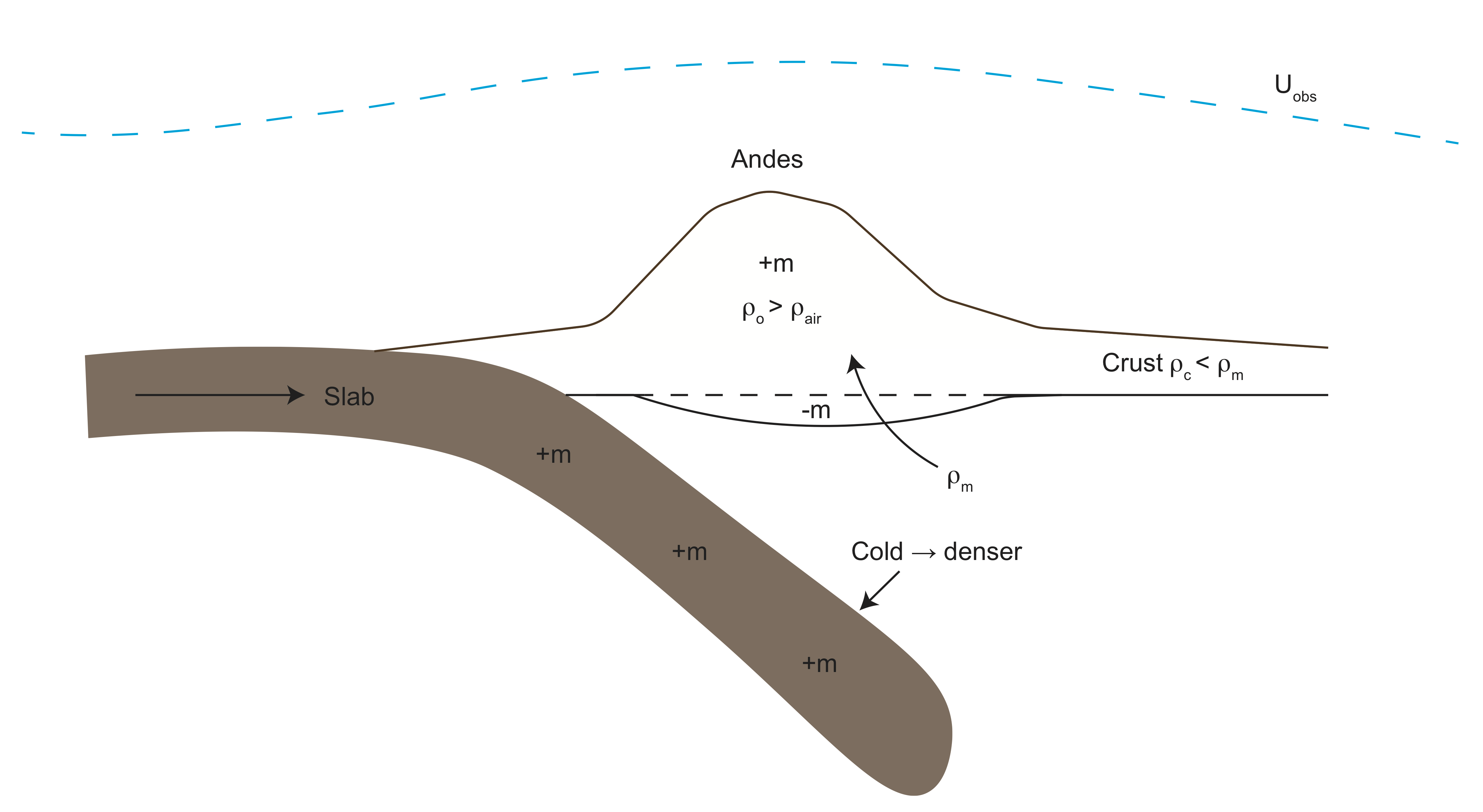
Second, the sinking of the slab will pull down on the surface creating a region of lower mass that compensates for the mass anomaly of the slab. In the Earth, the fact that the viscosity increases by about 30 x at around 660 km, means that the surface is not dragged down as much as it would be if the mantle had a uniform viscosity. So there is less compensation of the mass anomaly of the slab.
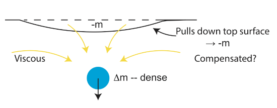
In summary, deformation (viscous flow and/or bending) in response to one mass anomaly can create mass anomalies of opposite sign. These are compensating anomalies. The gravitational field from all the mass anomalies sum up to give the total gravitational field. Gravity anomalies over compensated masses are much smaller (or zero) than the gravity anomaly of the initial mass anomaly.