4.6: Gyres and Surface Currents
- Page ID
- 14945
\( \newcommand{\vecs}[1]{\overset { \scriptstyle \rightharpoonup} {\mathbf{#1}} } \)
\( \newcommand{\vecd}[1]{\overset{-\!-\!\rightharpoonup}{\vphantom{a}\smash {#1}}} \)
\( \newcommand{\id}{\mathrm{id}}\) \( \newcommand{\Span}{\mathrm{span}}\)
( \newcommand{\kernel}{\mathrm{null}\,}\) \( \newcommand{\range}{\mathrm{range}\,}\)
\( \newcommand{\RealPart}{\mathrm{Re}}\) \( \newcommand{\ImaginaryPart}{\mathrm{Im}}\)
\( \newcommand{\Argument}{\mathrm{Arg}}\) \( \newcommand{\norm}[1]{\| #1 \|}\)
\( \newcommand{\inner}[2]{\langle #1, #2 \rangle}\)
\( \newcommand{\Span}{\mathrm{span}}\)
\( \newcommand{\id}{\mathrm{id}}\)
\( \newcommand{\Span}{\mathrm{span}}\)
\( \newcommand{\kernel}{\mathrm{null}\,}\)
\( \newcommand{\range}{\mathrm{range}\,}\)
\( \newcommand{\RealPart}{\mathrm{Re}}\)
\( \newcommand{\ImaginaryPart}{\mathrm{Im}}\)
\( \newcommand{\Argument}{\mathrm{Arg}}\)
\( \newcommand{\norm}[1]{\| #1 \|}\)
\( \newcommand{\inner}[2]{\langle #1, #2 \rangle}\)
\( \newcommand{\Span}{\mathrm{span}}\) \( \newcommand{\AA}{\unicode[.8,0]{x212B}}\)
\( \newcommand{\vectorA}[1]{\vec{#1}} % arrow\)
\( \newcommand{\vectorAt}[1]{\vec{\text{#1}}} % arrow\)
\( \newcommand{\vectorB}[1]{\overset { \scriptstyle \rightharpoonup} {\mathbf{#1}} } \)
\( \newcommand{\vectorC}[1]{\textbf{#1}} \)
\( \newcommand{\vectorD}[1]{\overrightarrow{#1}} \)
\( \newcommand{\vectorDt}[1]{\overrightarrow{\text{#1}}} \)
\( \newcommand{\vectE}[1]{\overset{-\!-\!\rightharpoonup}{\vphantom{a}\smash{\mathbf {#1}}}} \)
\( \newcommand{\vecs}[1]{\overset { \scriptstyle \rightharpoonup} {\mathbf{#1}} } \)
\( \newcommand{\vecd}[1]{\overset{-\!-\!\rightharpoonup}{\vphantom{a}\smash {#1}}} \)
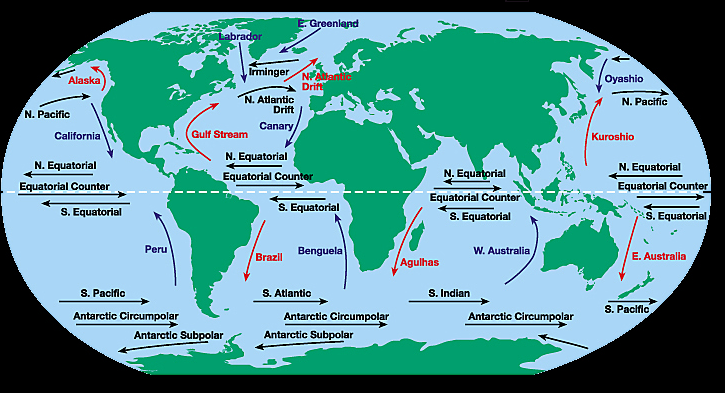
\(\newcommand{\avec}{\mathbf a}\) \(\newcommand{\bvec}{\mathbf b}\) \(\newcommand{\cvec}{\mathbf c}\) \(\newcommand{\dvec}{\mathbf d}\) \(\newcommand{\dtil}{\widetilde{\mathbf d}}\) \(\newcommand{\evec}{\mathbf e}\) \(\newcommand{\fvec}{\mathbf f}\) \(\newcommand{\nvec}{\mathbf n}\) \(\newcommand{\pvec}{\mathbf p}\) \(\newcommand{\qvec}{\mathbf q}\) \(\newcommand{\svec}{\mathbf s}\) \(\newcommand{\tvec}{\mathbf t}\) \(\newcommand{\uvec}{\mathbf u}\) \(\newcommand{\vvec}{\mathbf v}\) \(\newcommand{\wvec}{\mathbf w}\) \(\newcommand{\xvec}{\mathbf x}\) \(\newcommand{\yvec}{\mathbf y}\) \(\newcommand{\zvec}{\mathbf z}\) \(\newcommand{\rvec}{\mathbf r}\) \(\newcommand{\mvec}{\mathbf m}\) \(\newcommand{\zerovec}{\mathbf 0}\) \(\newcommand{\onevec}{\mathbf 1}\) \(\newcommand{\real}{\mathbb R}\) \(\newcommand{\twovec}[2]{\left[\begin{array}{r}#1 \\ #2 \end{array}\right]}\) \(\newcommand{\ctwovec}[2]{\left[\begin{array}{c}#1 \\ #2 \end{array}\right]}\) \(\newcommand{\threevec}[3]{\left[\begin{array}{r}#1 \\ #2 \\ #3 \end{array}\right]}\) \(\newcommand{\cthreevec}[3]{\left[\begin{array}{c}#1 \\ #2 \\ #3 \end{array}\right]}\) \(\newcommand{\fourvec}[4]{\left[\begin{array}{r}#1 \\ #2 \\ #3 \\ #4 \end{array}\right]}\) \(\newcommand{\cfourvec}[4]{\left[\begin{array}{c}#1 \\ #2 \\ #3 \\ #4 \end{array}\right]}\) \(\newcommand{\fivevec}[5]{\left[\begin{array}{r}#1 \\ #2 \\ #3 \\ #4 \\ #5 \\ \end{array}\right]}\) \(\newcommand{\cfivevec}[5]{\left[\begin{array}{c}#1 \\ #2 \\ #3 \\ #4 \\ #5 \\ \end{array}\right]}\) \(\newcommand{\mattwo}[4]{\left[\begin{array}{rr}#1 \amp #2 \\ #3 \amp #4 \\ \end{array}\right]}\) \(\newcommand{\laspan}[1]{\text{Span}\{#1\}}\) \(\newcommand{\bcal}{\cal B}\) \(\newcommand{\ccal}{\cal C}\) \(\newcommand{\scal}{\cal S}\) \(\newcommand{\wcal}{\cal W}\) \(\newcommand{\ecal}{\cal E}\) \(\newcommand{\coords}[2]{\left\{#1\right\}_{#2}}\) \(\newcommand{\gray}[1]{\color{gray}{#1}}\) \(\newcommand{\lgray}[1]{\color{lightgray}{#1}}\) \(\newcommand{\rank}{\operatorname{rank}}\) \(\newcommand{\row}{\text{Row}}\) \(\newcommand{\col}{\text{Col}}\) \(\renewcommand{\row}{\text{Row}}\) \(\newcommand{\nul}{\text{Nul}}\) \(\newcommand{\var}{\text{Var}}\) \(\newcommand{\corr}{\text{corr}}\) \(\newcommand{\len}[1]{\left|#1\right|}\) \(\newcommand{\bbar}{\overline{\bvec}}\) \(\newcommand{\bhat}{\widehat{\bvec}}\) \(\newcommand{\bperp}{\bvec^\perp}\) \(\newcommand{\xhat}{\widehat{\xvec}}\) \(\newcommand{\vhat}{\widehat{\vvec}}\) \(\newcommand{\uhat}{\widehat{\uvec}}\) \(\newcommand{\what}{\widehat{\wvec}}\) \(\newcommand{\Sighat}{\widehat{\Sigma}}\) \(\newcommand{\lt}{<}\) \(\newcommand{\gt}{>}\) \(\newcommand{\amp}{&}\) \(\definecolor{fillinmathshade}{gray}{0.9}\)The global pattern of winds together with the Coriolis Effect and Ekman Transport produce large-scale currents in the world ocean. Ocean surface currents organize into Gyres that are characterized by circulation at the scale of the ocean basin. The figure below shows the basic pattern. Note that gyres circulate clockwise in the northern Hemisphere and counter-clockwise in the Southern Hemisphere.

Source: UCAR
The influence of the Coriolis effect on ocean currents increases with increasing latitude, so the equatorial currents are similar in each ocean basin, although their flow direction (east to west) is consistent with the sense of flow in the large-scale gyres within each ocean basin. But the variation of Coriolis forcing as a function of latitude has a pronounced affect on surface currents. The poleward currents on the Western side of each ocean basin are distinctly different from those on the Eastern side of the ocean basin.
Western Boundary Currents are swift, narrow and deep relative to Eastern Boundary Currents, which are slower, broader and shallower than WBC's. Western Boundary Currents tend to carry heat from the equator poleward, so think back to where we started in this Lesson; everything is driven by differential solar heating. The excess heat received in the equatorial regions drives everything, including the strong Western Boundary Currents such as the familiar Gulf Stream and the East Australian Current (from Finding Nemo fame).
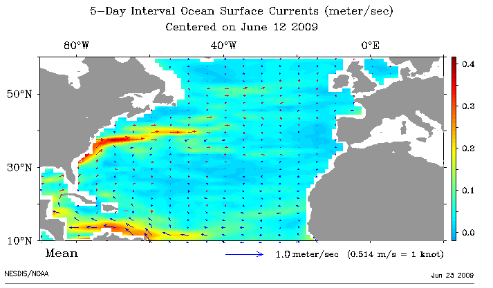
The figure below shows surface current information for the North Atlantic. The color scale is flow velocity in m/s, and the arrow along the bottom shows a 1 m/s scale bar (vector). Note the narrowness of the Gulf Stream.
Look here for more info on the Gulf Stream.(link is external)

Source: NOAA
Activity 3
Let's make our own maps and use them to calculate some things about heat transport. For this activity we will use ESR (Earth and Space Research) out of Seattle, WA. They have great research projects like OSCAR (Ocean Surface Current Analyses Real-Time) which suites our purposes nicely. Let's visit them HERE(link is external). There's some good background information about OSCAR there, but we will be using the link "OSCAR on SOTO", with SOTO standing for "State of the Ocean". Once you click on "OSCAR on SOTO", you will open up a really cool interactive map. I encourage you to play around with it for a bit to see what kind of data it is capable of conveying (we could have used this for our density calculations for Activity 2!) Once you're done playing, check out "Ocean Current Speed", but then settle on "Ocean Current Vectors".
->Note: This web site is mostly gone. Some of it is available here: https://www.esr.org/research/oscar/overview/(link is external)
- Make and save (using "Grab" on a Mac or another print-screen application) a few maps of surface currents where you look at seasonal variations as well as flow directions and the basic pattern of ocean-basin scale gyres.
- Choose your favorite map and tell me why you chose it in a few sentences. What did you learn from it? Put your map in a file, along with your comments.
- And now for a couple of calculations.
- Calculate an estimate of the volume of water that flowed poleward in the Gulf Stream during all of June 2016.
- Calculate an estimate of how much heat was transported by the Gulf Stream in June 2016 (You can choose to estimate sensible heat and/or latent heat)
There are multiple ways one can do these, just make sure I can follow your train of thought through each/both. Your calculations should:
- incorporate the max velocity of the Gulf Stream from June 2016
- assume that the depth of the current is 1 km
- estimate the width of the Gulf Stream from your map
- use OSCAR to find temperature estimates
Submitting your work
Please put your answers in a file and drop that in the dropbox for Activity 3 on Canvas.
Save your document as either a Microsoft Word or PDF file in the following format:
L4_Activity3_AccessAccountID_LastName.doc (or .pages or .pdf)
For example, student Elvis Aaron Presley's file would be named "L4_Activity3_eap1_presley.doc".
Grading criteria
See the grading rubric for specifics on how this assignment will be graded.


