10.2: Why are midlatitude winds mostly westerly (i.e., eastward)?
- Page ID
- 6553
\( \newcommand{\vecs}[1]{\overset { \scriptstyle \rightharpoonup} {\mathbf{#1}} } \)
\( \newcommand{\vecd}[1]{\overset{-\!-\!\rightharpoonup}{\vphantom{a}\smash {#1}}} \)
\( \newcommand{\id}{\mathrm{id}}\) \( \newcommand{\Span}{\mathrm{span}}\)
( \newcommand{\kernel}{\mathrm{null}\,}\) \( \newcommand{\range}{\mathrm{range}\,}\)
\( \newcommand{\RealPart}{\mathrm{Re}}\) \( \newcommand{\ImaginaryPart}{\mathrm{Im}}\)
\( \newcommand{\Argument}{\mathrm{Arg}}\) \( \newcommand{\norm}[1]{\| #1 \|}\)
\( \newcommand{\inner}[2]{\langle #1, #2 \rangle}\)
\( \newcommand{\Span}{\mathrm{span}}\)
\( \newcommand{\id}{\mathrm{id}}\)
\( \newcommand{\Span}{\mathrm{span}}\)
\( \newcommand{\kernel}{\mathrm{null}\,}\)
\( \newcommand{\range}{\mathrm{range}\,}\)
\( \newcommand{\RealPart}{\mathrm{Re}}\)
\( \newcommand{\ImaginaryPart}{\mathrm{Im}}\)
\( \newcommand{\Argument}{\mathrm{Arg}}\)
\( \newcommand{\norm}[1]{\| #1 \|}\)
\( \newcommand{\inner}[2]{\langle #1, #2 \rangle}\)
\( \newcommand{\Span}{\mathrm{span}}\) \( \newcommand{\AA}{\unicode[.8,0]{x212B}}\)
\( \newcommand{\vectorA}[1]{\vec{#1}} % arrow\)
\( \newcommand{\vectorAt}[1]{\vec{\text{#1}}} % arrow\)
\( \newcommand{\vectorB}[1]{\overset { \scriptstyle \rightharpoonup} {\mathbf{#1}} } \)
\( \newcommand{\vectorC}[1]{\textbf{#1}} \)
\( \newcommand{\vectorD}[1]{\overrightarrow{#1}} \)
\( \newcommand{\vectorDt}[1]{\overrightarrow{\text{#1}}} \)
\( \newcommand{\vectE}[1]{\overset{-\!-\!\rightharpoonup}{\vphantom{a}\smash{\mathbf {#1}}}} \)
\( \newcommand{\vecs}[1]{\overset { \scriptstyle \rightharpoonup} {\mathbf{#1}} } \)
\( \newcommand{\vecd}[1]{\overset{-\!-\!\rightharpoonup}{\vphantom{a}\smash {#1}}} \)
\(\newcommand{\avec}{\mathbf a}\) \(\newcommand{\bvec}{\mathbf b}\) \(\newcommand{\cvec}{\mathbf c}\) \(\newcommand{\dvec}{\mathbf d}\) \(\newcommand{\dtil}{\widetilde{\mathbf d}}\) \(\newcommand{\evec}{\mathbf e}\) \(\newcommand{\fvec}{\mathbf f}\) \(\newcommand{\nvec}{\mathbf n}\) \(\newcommand{\pvec}{\mathbf p}\) \(\newcommand{\qvec}{\mathbf q}\) \(\newcommand{\svec}{\mathbf s}\) \(\newcommand{\tvec}{\mathbf t}\) \(\newcommand{\uvec}{\mathbf u}\) \(\newcommand{\vvec}{\mathbf v}\) \(\newcommand{\wvec}{\mathbf w}\) \(\newcommand{\xvec}{\mathbf x}\) \(\newcommand{\yvec}{\mathbf y}\) \(\newcommand{\zvec}{\mathbf z}\) \(\newcommand{\rvec}{\mathbf r}\) \(\newcommand{\mvec}{\mathbf m}\) \(\newcommand{\zerovec}{\mathbf 0}\) \(\newcommand{\onevec}{\mathbf 1}\) \(\newcommand{\real}{\mathbb R}\) \(\newcommand{\twovec}[2]{\left[\begin{array}{r}#1 \\ #2 \end{array}\right]}\) \(\newcommand{\ctwovec}[2]{\left[\begin{array}{c}#1 \\ #2 \end{array}\right]}\) \(\newcommand{\threevec}[3]{\left[\begin{array}{r}#1 \\ #2 \\ #3 \end{array}\right]}\) \(\newcommand{\cthreevec}[3]{\left[\begin{array}{c}#1 \\ #2 \\ #3 \end{array}\right]}\) \(\newcommand{\fourvec}[4]{\left[\begin{array}{r}#1 \\ #2 \\ #3 \\ #4 \end{array}\right]}\) \(\newcommand{\cfourvec}[4]{\left[\begin{array}{c}#1 \\ #2 \\ #3 \\ #4 \end{array}\right]}\) \(\newcommand{\fivevec}[5]{\left[\begin{array}{r}#1 \\ #2 \\ #3 \\ #4 \\ #5 \\ \end{array}\right]}\) \(\newcommand{\cfivevec}[5]{\left[\begin{array}{c}#1 \\ #2 \\ #3 \\ #4 \\ #5 \\ \end{array}\right]}\) \(\newcommand{\mattwo}[4]{\left[\begin{array}{rr}#1 \amp #2 \\ #3 \amp #4 \\ \end{array}\right]}\) \(\newcommand{\laspan}[1]{\text{Span}\{#1\}}\) \(\newcommand{\bcal}{\cal B}\) \(\newcommand{\ccal}{\cal C}\) \(\newcommand{\scal}{\cal S}\) \(\newcommand{\wcal}{\cal W}\) \(\newcommand{\ecal}{\cal E}\) \(\newcommand{\coords}[2]{\left\{#1\right\}_{#2}}\) \(\newcommand{\gray}[1]{\color{gray}{#1}}\) \(\newcommand{\lgray}[1]{\color{lightgray}{#1}}\) \(\newcommand{\rank}{\operatorname{rank}}\) \(\newcommand{\row}{\text{Row}}\) \(\newcommand{\col}{\text{Col}}\) \(\renewcommand{\row}{\text{Row}}\) \(\newcommand{\nul}{\text{Nul}}\) \(\newcommand{\var}{\text{Var}}\) \(\newcommand{\corr}{\text{corr}}\) \(\newcommand{\len}[1]{\left|#1\right|}\) \(\newcommand{\bbar}{\overline{\bvec}}\) \(\newcommand{\bhat}{\widehat{\bvec}}\) \(\newcommand{\bperp}{\bvec^\perp}\) \(\newcommand{\xhat}{\widehat{\xvec}}\) \(\newcommand{\vhat}{\widehat{\vvec}}\) \(\newcommand{\uhat}{\widehat{\uvec}}\) \(\newcommand{\what}{\widehat{\wvec}}\) \(\newcommand{\Sighat}{\widehat{\Sigma}}\) \(\newcommand{\lt}{<}\) \(\newcommand{\gt}{>}\) \(\newcommand{\amp}{&}\) \(\definecolor{fillinmathshade}{gray}{0.9}\)The answer seems simple. More solar energy is deposited in the tropics than near the poles and as a result, the air is warmer in the tropics than the poles, where there is net radiative cooling. According to the hydrostatic equilibrium equation, the fall-off in pressure with altitude is less in the tropics than at higher latitudes, and as a result, for any height surface, the pressure is greater in the tropics than near the poles, setting up a pressure gradient force on each height surface that drives the wind poleward. As the air moves poleward, atmospheric processes such as the Coriolis force, which we saw occurs because of conservation of angular momentum, and synoptic-scale disturbances at higher latitudes cause the air to veer to the right in the Northern Hemisphere and to the left in the Southern Hemisphere.
Thermal Wind
With this broad concept in mind, we can consider the idea of the thermal wind, which is not really a wind, but instead is a difference in winds at two heights. We will see that the thermal wind is proportional to the horizontal temperature gradient. To show this relationship mathematically, we start with the geostrophic balance equation and apply the Ideal Gas Law and the hydrostatic equilibrium equation.
Look at the x and y components of Equation [10.33] for geostrophic winds:
\[v_{g}=\frac{1}{f} \frac{\partial \Phi}{\partial x}\]
\[u_{g}=-\frac{1}{f} \frac{\partial \Phi}{\partial y}\]
Use the hydrostatic equation and the Ideal Gas Law to relate T to Φ:
\(\frac{\partial p}{\partial z}=-\rho g \quad \rightarrow \quad \frac{\partial p}{g \partial z}=-\rho \quad \rightarrow \quad \frac{\partial p}{\partial \Phi}=-\rho \quad \rightarrow \quad \frac{\partial \Phi}{\partial p}=-\frac{1}{\rho}=-\frac{R T}{p}\)
Take \(\frac{\partial}{\partial p}\) of equations in [10.41], starting with the equation for \(\mathcal{V}_{\mathcal{G}}\):
\[\frac{\partial v_{g}}{\partial p}=\frac{1}{f} \frac{\partial}{\partial p}\left(\frac{\partial \Phi}{\partial x}\right)=\frac{1}{f} \frac{\partial}{\partial x}\left(\frac{\partial \Phi}{\partial p}\right)=\frac{1}{f} \frac{\partial}{\partial x}\left(-\frac{R T}{p}\right)\]
\[p \frac{\partial v_{g}}{\partial p}=-\frac{R}{f} \frac{\partial T}{\partial x} \quad\) and \(\quad p \frac{\partial v_{g}}{\partial p}=\frac{\partial v_{g}}{\partial \ln p}\]
Taking the same approach with the equation for ugug gives the Thermal Wind Equations:
\[\frac{\partial v_{g}}{\partial \ln p}=-\frac{R}{f}\left(\frac{\partial T}{\partial x}\right)_{p}\] and \[\frac{\partial u_{g}}{\partial \ln p}=\frac{R}{f}\left(\frac{\partial T}{\partial y}\right)_{p}\]
\[\frac{\partial \vec{V}_{g}}{\partial \ln p}=-\frac{R}{f} \vec{k} \times \vec{\nabla}_{p} T \quad\] in vector form
These equations are very powerful because they reveal that measurements of temperature only (which are relatively easy to make) make it possible to determine the changes in the horizontal wind with height, assuming that the geostrophic and hydrostatic approximations are valid (which is the case for large-scale flow in the free atmosphere). The thermal wind velocity is defined as the change in horizontal geostrophic velocity between two layers.
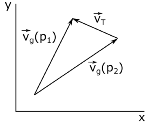
\[\vec{V}_{T} \equiv \vec{V}_{g}\left(p_{1}\right)-\vec{V}_{g}\left(p_{2}\right), \quad p_{1}<p_{2}\]
So the thermal wind velocity equals the horizontal velocity at the upper level minus the horizontal velocity at the lower level. Equation [10.43] can be drawn as a two-dimensional vector subtraction as if we were looking down on them from above (see figure below).

We can integrate Equation [10.42] and if we let <T> be the average temperature between pressure surfaces p1 and p2 (where p1 < p2), yielding the expressions for the thermal wind vectors in the x and y directions:
\[\vec{V}_{T}=u_{T} \vec{i}+v_{T} \vec{j}=\frac{R}{f}\left[\vec{j}\left(\frac{\partial\langle T\rangle}{\partial x}\right)_{p}-\vec{i}\left(\frac{\partial\langle T\rangle}{\partial y}\right)_{p}\right] \ln \left(\frac{p_{2}}{p_{1}}\right)\]
\[\vec{V}_{T}=\frac{R}{f} \ln \left(\frac{p_{2}}{p_{1}}\right) \vec{k} \times \vec{\nabla}_{p}\langle T\rangle\]
\[u_{T}=-\frac{R}{f}\left(\frac{\partial\langle T\rangle}{\partial y}\right)_{p} \ln \left(\frac{p_{2}}{p_{1}}\right)\] \[v_{T}=\frac{R}{f}\left(\frac{\partial\langle T\rangle}{\partial x}\right)_{p} \ln \left(\frac{p_{2}}{p_{1}}\right)\]
The vertical change in geostrophic wind is called the geostrophic vertical shear. Since the geostrophic vertical shear is directly proportional to the horizontal temperature gradient, it is also called the Thermal Wind.

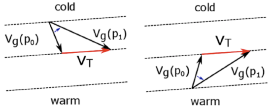
Thermal wind is the vector difference of the geostrophic wind at the upper-level pressure (p1) minus the lower-level pressure (p0, which should be written as p2 to be consistent with the previous figure and the text). These figures show the view looking down on the x-y plane. Cold air is on the left of VT. Left: Backing (flow turning counterclockwise with height) indicates cold advection. Right: Veering (flow turning clockwise with height) indicates warm air advection. Credit: W. Brune
We can learn a lot from the thermal wind (seen in the figure above).
- Thermal wind blows with cold air to the left (on average) and with the warm air on the right in the Northern Hemisphere (remember “air is light on the right”), and with warm air on the left in the Southern Hemisphere.
- If the geostrophic wind vector rotates counterclockwise with height (called backing), then there is cold air advection. For the Northern Hemisphere, remember “CCC: counterclockwise cold.”
- If the geostrophic wind vector rotates clockwise with height (called veering), then there is warm air advection.
- In the Northern Hemisphere, because low thickness means lower layer temperature and higher thickness means higher layer temperature, the thermal wind blows parallel to the lines of constant thickness with the low thickness on the left.
- This statement is an analogy to “The geostrophic wind blows parallel to the height contours on a pressure surface (pressure contours on a height surface) with the low height (pressure) to the left."
Quiz 10-4: Feeling the thermal wind.
- Find Practice Quiz 10-4 in Canvas. You may complete this practice quiz as many times as you want. It is not graded, but it allows you to check your level of preparedness before taking the graded quiz.
- When you feel you are ready, take Quiz 10-4. You will be allowed to take this quiz only once. Good luck!

