
2.10: Lab 10 - Fold and Thrust Belts
- Page ID
- 12523

\( \newcommand{\vecs}[1]{\overset { \scriptstyle \rightharpoonup} {\mathbf{#1}} } \)
\( \newcommand{\vecd}[1]{\overset{-\!-\!\rightharpoonup}{\vphantom{a}\smash {#1}}} \)
\( \newcommand{\id}{\mathrm{id}}\) \( \newcommand{\Span}{\mathrm{span}}\)
( \newcommand{\kernel}{\mathrm{null}\,}\) \( \newcommand{\range}{\mathrm{range}\,}\)
\( \newcommand{\RealPart}{\mathrm{Re}}\) \( \newcommand{\ImaginaryPart}{\mathrm{Im}}\)
\( \newcommand{\Argument}{\mathrm{Arg}}\) \( \newcommand{\norm}[1]{\| #1 \|}\)
\( \newcommand{\inner}[2]{\langle #1, #2 \rangle}\)
\( \newcommand{\Span}{\mathrm{span}}\)
\( \newcommand{\id}{\mathrm{id}}\)
\( \newcommand{\Span}{\mathrm{span}}\)
\( \newcommand{\kernel}{\mathrm{null}\,}\)
\( \newcommand{\range}{\mathrm{range}\,}\)
\( \newcommand{\RealPart}{\mathrm{Re}}\)
\( \newcommand{\ImaginaryPart}{\mathrm{Im}}\)
\( \newcommand{\Argument}{\mathrm{Arg}}\)
\( \newcommand{\norm}[1]{\| #1 \|}\)
\( \newcommand{\inner}[2]{\langle #1, #2 \rangle}\)
\( \newcommand{\Span}{\mathrm{span}}\) \( \newcommand{\AA}{\unicode[.8,0]{x212B}}\)
\( \newcommand{\vectorA}[1]{\vec{#1}} % arrow\)
\( \newcommand{\vectorAt}[1]{\vec{\text{#1}}} % arrow\)
\( \newcommand{\vectorB}[1]{\overset { \scriptstyle \rightharpoonup} {\mathbf{#1}} } \)
\( \newcommand{\vectorC}[1]{\textbf{#1}} \)
\( \newcommand{\vectorD}[1]{\overrightarrow{#1}} \)
\( \newcommand{\vectorDt}[1]{\overrightarrow{\text{#1}}} \)
\( \newcommand{\vectE}[1]{\overset{-\!-\!\rightharpoonup}{\vphantom{a}\smash{\mathbf {#1}}}} \)
\( \newcommand{\vecs}[1]{\overset { \scriptstyle \rightharpoonup} {\mathbf{#1}} } \)
\( \newcommand{\vecd}[1]{\overset{-\!-\!\rightharpoonup}{\vphantom{a}\smash {#1}}} \)
\(\newcommand{\avec}{\mathbf a}\) \(\newcommand{\bvec}{\mathbf b}\) \(\newcommand{\cvec}{\mathbf c}\) \(\newcommand{\dvec}{\mathbf d}\) \(\newcommand{\dtil}{\widetilde{\mathbf d}}\) \(\newcommand{\evec}{\mathbf e}\) \(\newcommand{\fvec}{\mathbf f}\) \(\newcommand{\nvec}{\mathbf n}\) \(\newcommand{\pvec}{\mathbf p}\) \(\newcommand{\qvec}{\mathbf q}\) \(\newcommand{\svec}{\mathbf s}\) \(\newcommand{\tvec}{\mathbf t}\) \(\newcommand{\uvec}{\mathbf u}\) \(\newcommand{\vvec}{\mathbf v}\) \(\newcommand{\wvec}{\mathbf w}\) \(\newcommand{\xvec}{\mathbf x}\) \(\newcommand{\yvec}{\mathbf y}\) \(\newcommand{\zvec}{\mathbf z}\) \(\newcommand{\rvec}{\mathbf r}\) \(\newcommand{\mvec}{\mathbf m}\) \(\newcommand{\zerovec}{\mathbf 0}\) \(\newcommand{\onevec}{\mathbf 1}\) \(\newcommand{\real}{\mathbb R}\) \(\newcommand{\twovec}[2]{\left[\begin{array}{r}#1 \\ #2 \end{array}\right]}\) \(\newcommand{\ctwovec}[2]{\left[\begin{array}{c}#1 \\ #2 \end{array}\right]}\) \(\newcommand{\threevec}[3]{\left[\begin{array}{r}#1 \\ #2 \\ #3 \end{array}\right]}\) \(\newcommand{\cthreevec}[3]{\left[\begin{array}{c}#1 \\ #2 \\ #3 \end{array}\right]}\) \(\newcommand{\fourvec}[4]{\left[\begin{array}{r}#1 \\ #2 \\ #3 \\ #4 \end{array}\right]}\) \(\newcommand{\cfourvec}[4]{\left[\begin{array}{c}#1 \\ #2 \\ #3 \\ #4 \end{array}\right]}\) \(\newcommand{\fivevec}[5]{\left[\begin{array}{r}#1 \\ #2 \\ #3 \\ #4 \\ #5 \\ \end{array}\right]}\) \(\newcommand{\cfivevec}[5]{\left[\begin{array}{c}#1 \\ #2 \\ #3 \\ #4 \\ #5 \\ \end{array}\right]}\) \(\newcommand{\mattwo}[4]{\left[\begin{array}{rr}#1 \amp #2 \\ #3 \amp #4 \\ \end{array}\right]}\) \(\newcommand{\laspan}[1]{\text{Span}\{#1\}}\) \(\newcommand{\bcal}{\cal B}\) \(\newcommand{\ccal}{\cal C}\) \(\newcommand{\scal}{\cal S}\) \(\newcommand{\wcal}{\cal W}\) \(\newcommand{\ecal}{\cal E}\) \(\newcommand{\coords}[2]{\left\{#1\right\}_{#2}}\) \(\newcommand{\gray}[1]{\color{gray}{#1}}\) \(\newcommand{\lgray}[1]{\color{lightgray}{#1}}\) \(\newcommand{\rank}{\operatorname{rank}}\) \(\newcommand{\row}{\text{Row}}\) \(\newcommand{\col}{\text{Col}}\) \(\renewcommand{\row}{\text{Row}}\) \(\newcommand{\nul}{\text{Nul}}\) \(\newcommand{\var}{\text{Var}}\) \(\newcommand{\corr}{\text{corr}}\) \(\newcommand{\len}[1]{\left|#1\right|}\) \(\newcommand{\bbar}{\overline{\bvec}}\) \(\newcommand{\bhat}{\widehat{\bvec}}\) \(\newcommand{\bperp}{\bvec^\perp}\) \(\newcommand{\xhat}{\widehat{\xvec}}\) \(\newcommand{\vhat}{\widehat{\vvec}}\) \(\newcommand{\uhat}{\widehat{\uvec}}\) \(\newcommand{\what}{\widehat{\wvec}}\) \(\newcommand{\Sighat}{\widehat{\Sigma}}\) \(\newcommand{\lt}{<}\) \(\newcommand{\gt}{>}\) \(\newcommand{\amp}{&}\) \(\definecolor{fillinmathshade}{gray}{0.9}\)Introduction
The Foothills, Front Ranges and Main Ranges of the Canadian Cordillera are one of the world’s best described fold and thrust belts, in which sedimentary strata have been shortened by hundreds of kilometres while remaining at low temperature and showing, at most, low grade metamorphism. Other examples of fold and thrust belts include the Appalachian Valley and Ridge province the eastern U.S., the Jura Mountains in the Swiss Alps, and the Moine Thrust zone in NW Scotland. Many of these belts contain substantial reservoirs of oil and natural gas in structural traps, and therefore considerable effort has gone into understanding their geometry and kinematics.
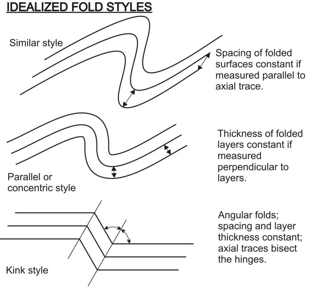
Because of the relatively low temperatures at which the rocks were deformed, there are strong contrasts between competent lithologies (typically limestones and sandstones) and incompetent lithologies (typically shales and evaporites). As a result, faults tend to follow ramp–flat trajectories through the stratigraphy, and most folds are related to variations in the slip or dip of faults (or both). Also, competent lithologies tend to be translated large distances without large amounts of internal distortion, except at the hinges of folds. Therefore, fold and thrust belts often show layers that maintain their original thicknesses; folds of this style are called parallel folds (Fig. 1). These properties are helpful in the construction of cross-sections, especially in areas where the sheer number of faults and folds make conventional structure contouring difficult.
Techniques for folds in profile
In the first part of this lab, you will explore two techniques for constructing cross-sections through subhorizontal folds that are useful in preliminary work on thrust-related folds.
Parallel folds are also sometimes called concentric folds, because the curved arcs are parallel, and are centred on common centres. When a stack of layers exhibits this special geometry, it is possible to make predictions of the continuation of structures at depth that assist with cross-section construction. We will use the Busk or Arcconstruction to reconstruct the folds. This construction assumes folds are cylindrical and horizontal folds and the layers have concentric geometry. The first few steps in this technique are illustrated in Figures 2 and 3. There is also a helpful tutorial on the worldwide web at the website of Steven Dutch (University of Wisconsin):
- Arc method: stevedutch.net/Structge/SL161ArcMethod.htm
In some fold and thrust belts, it has been shown that instead of displaying smooth arcs like those postulated in the Busk construction, folds display straight limbs and angular hinges, like kink folds. This observation leads to the kink construction, in which folds are assumed to have straight limbs and angular hinges. Because beds have the same thickness on opposite limbs of each fold, the axial surfaces exactly bisect the inter-limb angles. In the kink construction, rounded fold hinges are approximated by multiple angular folds. Although kink folds depart from parallel geometry at the hinges, these hinge regions are very narrow; as a result, sometimes the kink and Busk constructions give rather similar results. First steps in the construction are illustrated in Figures 4 and 5. There is also a helpful tutorial on the worldwide web at the website of Steven Dutch (University of Wisconsin). Note, however, that the tutorial makes different assumptions about the locations of fold hinges, compared with the exercise in the assignment, where fold hinges are explicitly located.
- Kink Method: stevedutch.net/…uctge/SL162KinkMethod.htm
Assignment
- *Busk construction for parallel folds in profile cross-section
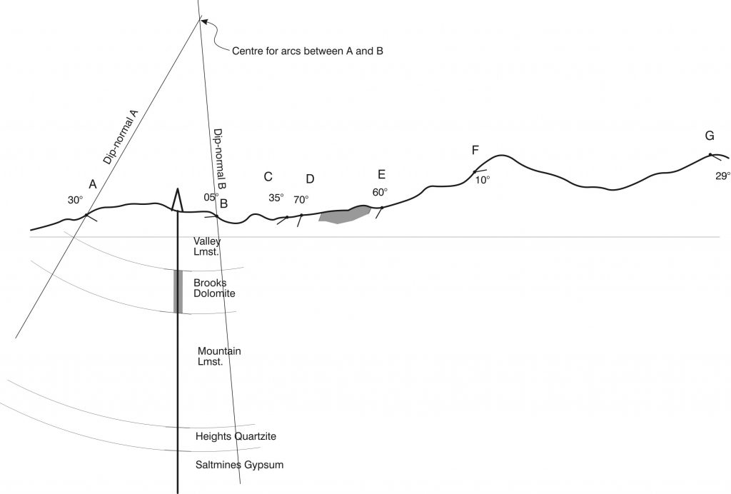
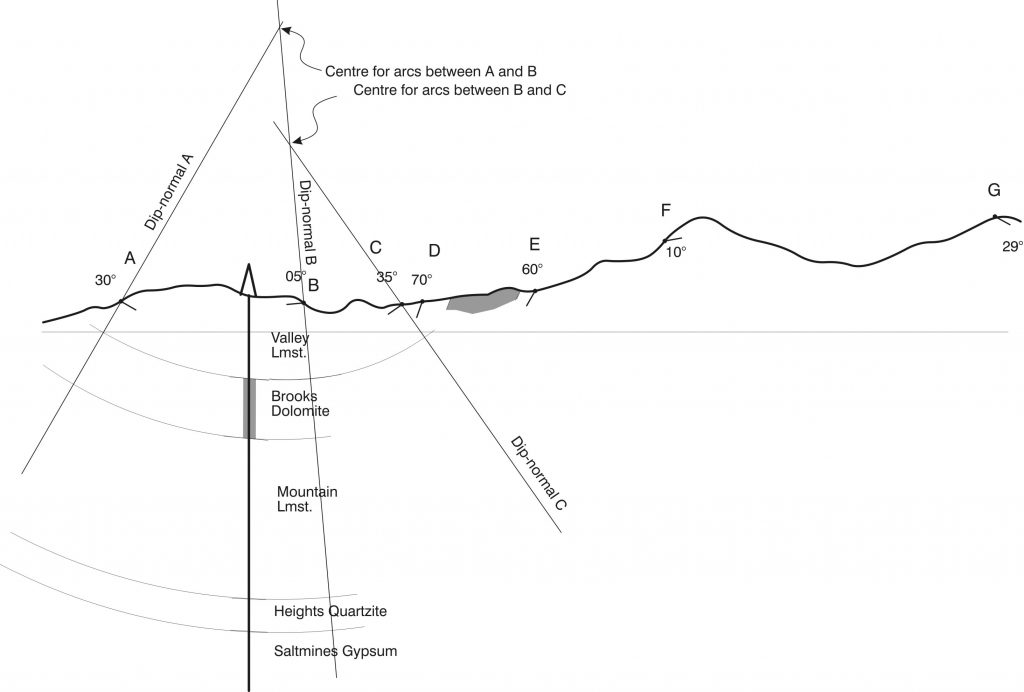
You are provided with a cross-section through an area of horizontal cylindrical folds, with subsurface information from a single borehole. The scale is 1:10,000, without vertical exaggeration. Dip measurements are shown at intervals at ground level. Make a cross-section using the Busk, or arc construction.
-
- To execute the Busk construction, draw a line perpendicular to the dip at each point where the dip was measured. (Use a protractor and the numerical value of dip from the section.) These lines are called dip normals. Give them letters A, B, C, etc.
- Find a place where there is stratigraphic information located between two adjacent dip normals e.g. between A and B. Use a compass with its point placed on the intersection of the bedding normals to extend the stratigraphic boundaries as far as those normals.
- Continue with the next pair of dip normals, using a compass to extend the boundaries, until the section is complete. You may assume that the strata beyond the right-hand end of the section dip at a constant 29°.
- The borehole is extended and encounters the base of the Saltmines Gypsum, which is 450 m thick. Add the base of the Gypsum to the cross section. Notice how the assumption of parallel folding breaks down at depth. (You may find it easiest to start at both ends of the section, measuring the 450 m of gypsum perpendicular to bedding in each case, and working toward the ‘difficult’ part in the centre.) Why would you expect the gypsum to behave differently?
Lab 10. Question 1. Busk Construction
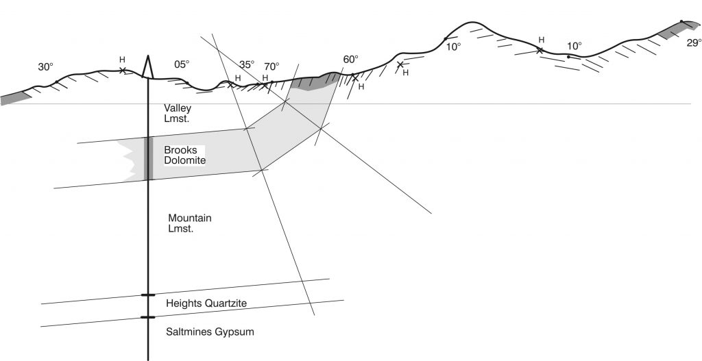
- *Kink construction for angular folds in profile cross-section
You are provided a second cross section that shows some additional information in the area of the previous exercise. A reconnaissance traverse has shown that dip domains are separated by angular folds. The hinges of these folds are marked ‘H’ with a small x symbol. The new traverse also detected the presence of Brooks Dolomite at both extreme ends of the section.
-
- At each fold hinge, construct an axial trace that bisects the bedding dips on either side. the easiest way to do this is to add the two dips, and divide by 2; this gives the angle from vertical of the bisector. (Be careful if the dips are in opposite directions; you will need to count one as negative and the other as positive.)
- Then draw the stratigraphic boundaries on either side of the axial trace; you should find that the thickness of each unit is unchanged as it crosses the fold. Complete the cross-section as before. Make sure you add the base of the Gypsum as before.
Lab 10. Question 2. Kink Construction
- Thrust belt cross-section
Map 1 represents a faulted and folded area in a thrust belt. Using the relationships between outcrop shape and topography, structure contours, and fault-bedding intersection lines (cut-off lines), your objective is to determine the structure of the area and construct an accurate cross-section along the marked line.
a) Preliminary examination of the map
Look at the outcrop pattern. Both the stratigraphic units and the faults generally have sinuous outcrop patterns that roughly follow contours in parts of the map, suggesting that in these areas both the faults and the stratigraphic units mostly have gentle dips. The repetition of stratigraphic units suggest a dipping fault has caused repetition of stratigraphy. The patterns of faults and outcrops on either side of the main valleys are rough mirror images of each other, suggesting that the valleys have been eroded through structures that are now exposed in both valley sides. Any thrust belt map has a lot of surfaces. Identify the major stratigraphic boundaries and faults with colours as you have done in previous maps. Use red for faults, blues, greens and browns for stratigraphic surfaces.
b) Cut-off lines
A useful first step is to identify cut-off points, where faults intersect stratigraphic units, and connect them, where possible, to draw cut-off lines. Remember that for each surface cut by a fault, there will be a hanging wall cut-off line and a footwall cut-off line. You may notice that corresponding cut-off points have similar elevations on each side of the main valleys. This suggests that the cut-off lines are almost horizontal. Draw possible cut-off lines on the map.
c) Structure contours
Now try to draw structure contours on the dipping surfaces. Note that, because we are in a thrust belt, that surfaces may be repeated, so you may have more than one set of contours on the same surface.
Try to use the minimum number of lines to build the cross-section; however if your map becomes cluttered and difficult to understand, you may wish to use tracing paper for some of the contour sets. Make sure you record the position of the corners of the base map on your tracing paper so that it can easily be located, but do not attempt to trace all the detail from the map onto your tracing paper.
d) Cross-section
Project all these lines onto the cross section and complete the most reasonable hypothesis you can for the overall structure on the cross section. Except where you have direct evidence to the contrary, assume a geometry in which layers maintain constant thickness (either a ‘Busk’ or a ‘kink’ geometry will do, or a freehand compromise between the two. Your layers should not visibly change thickness across the section.)
Lab 10. Map 1. Fold and thrust belt (revised version)