1.10: Photogrammetry and Structure-from-Motion
- Page ID
- 17281

\( \newcommand{\vecs}[1]{\overset { \scriptstyle \rightharpoonup} {\mathbf{#1}} } \)
\( \newcommand{\vecd}[1]{\overset{-\!-\!\rightharpoonup}{\vphantom{a}\smash {#1}}} \)
\( \newcommand{\dsum}{\displaystyle\sum\limits} \)
\( \newcommand{\dint}{\displaystyle\int\limits} \)
\( \newcommand{\dlim}{\displaystyle\lim\limits} \)
\( \newcommand{\id}{\mathrm{id}}\) \( \newcommand{\Span}{\mathrm{span}}\)
( \newcommand{\kernel}{\mathrm{null}\,}\) \( \newcommand{\range}{\mathrm{range}\,}\)
\( \newcommand{\RealPart}{\mathrm{Re}}\) \( \newcommand{\ImaginaryPart}{\mathrm{Im}}\)
\( \newcommand{\Argument}{\mathrm{Arg}}\) \( \newcommand{\norm}[1]{\| #1 \|}\)
\( \newcommand{\inner}[2]{\langle #1, #2 \rangle}\)
\( \newcommand{\Span}{\mathrm{span}}\)
\( \newcommand{\id}{\mathrm{id}}\)
\( \newcommand{\Span}{\mathrm{span}}\)
\( \newcommand{\kernel}{\mathrm{null}\,}\)
\( \newcommand{\range}{\mathrm{range}\,}\)
\( \newcommand{\RealPart}{\mathrm{Re}}\)
\( \newcommand{\ImaginaryPart}{\mathrm{Im}}\)
\( \newcommand{\Argument}{\mathrm{Arg}}\)
\( \newcommand{\norm}[1]{\| #1 \|}\)
\( \newcommand{\inner}[2]{\langle #1, #2 \rangle}\)
\( \newcommand{\Span}{\mathrm{span}}\) \( \newcommand{\AA}{\unicode[.8,0]{x212B}}\)
\( \newcommand{\vectorA}[1]{\vec{#1}} % arrow\)
\( \newcommand{\vectorAt}[1]{\vec{\text{#1}}} % arrow\)
\( \newcommand{\vectorB}[1]{\overset { \scriptstyle \rightharpoonup} {\mathbf{#1}} } \)
\( \newcommand{\vectorC}[1]{\textbf{#1}} \)
\( \newcommand{\vectorD}[1]{\overrightarrow{#1}} \)
\( \newcommand{\vectorDt}[1]{\overrightarrow{\text{#1}}} \)
\( \newcommand{\vectE}[1]{\overset{-\!-\!\rightharpoonup}{\vphantom{a}\smash{\mathbf {#1}}}} \)
\( \newcommand{\vecs}[1]{\overset { \scriptstyle \rightharpoonup} {\mathbf{#1}} } \)
\(\newcommand{\longvect}{\overrightarrow}\)
\( \newcommand{\vecd}[1]{\overset{-\!-\!\rightharpoonup}{\vphantom{a}\smash {#1}}} \)
\(\newcommand{\avec}{\mathbf a}\) \(\newcommand{\bvec}{\mathbf b}\) \(\newcommand{\cvec}{\mathbf c}\) \(\newcommand{\dvec}{\mathbf d}\) \(\newcommand{\dtil}{\widetilde{\mathbf d}}\) \(\newcommand{\evec}{\mathbf e}\) \(\newcommand{\fvec}{\mathbf f}\) \(\newcommand{\nvec}{\mathbf n}\) \(\newcommand{\pvec}{\mathbf p}\) \(\newcommand{\qvec}{\mathbf q}\) \(\newcommand{\svec}{\mathbf s}\) \(\newcommand{\tvec}{\mathbf t}\) \(\newcommand{\uvec}{\mathbf u}\) \(\newcommand{\vvec}{\mathbf v}\) \(\newcommand{\wvec}{\mathbf w}\) \(\newcommand{\xvec}{\mathbf x}\) \(\newcommand{\yvec}{\mathbf y}\) \(\newcommand{\zvec}{\mathbf z}\) \(\newcommand{\rvec}{\mathbf r}\) \(\newcommand{\mvec}{\mathbf m}\) \(\newcommand{\zerovec}{\mathbf 0}\) \(\newcommand{\onevec}{\mathbf 1}\) \(\newcommand{\real}{\mathbb R}\) \(\newcommand{\twovec}[2]{\left[\begin{array}{r}#1 \\ #2 \end{array}\right]}\) \(\newcommand{\ctwovec}[2]{\left[\begin{array}{c}#1 \\ #2 \end{array}\right]}\) \(\newcommand{\threevec}[3]{\left[\begin{array}{r}#1 \\ #2 \\ #3 \end{array}\right]}\) \(\newcommand{\cthreevec}[3]{\left[\begin{array}{c}#1 \\ #2 \\ #3 \end{array}\right]}\) \(\newcommand{\fourvec}[4]{\left[\begin{array}{r}#1 \\ #2 \\ #3 \\ #4 \end{array}\right]}\) \(\newcommand{\cfourvec}[4]{\left[\begin{array}{c}#1 \\ #2 \\ #3 \\ #4 \end{array}\right]}\) \(\newcommand{\fivevec}[5]{\left[\begin{array}{r}#1 \\ #2 \\ #3 \\ #4 \\ #5 \\ \end{array}\right]}\) \(\newcommand{\cfivevec}[5]{\left[\begin{array}{c}#1 \\ #2 \\ #3 \\ #4 \\ #5 \\ \end{array}\right]}\) \(\newcommand{\mattwo}[4]{\left[\begin{array}{rr}#1 \amp #2 \\ #3 \amp #4 \\ \end{array}\right]}\) \(\newcommand{\laspan}[1]{\text{Span}\{#1\}}\) \(\newcommand{\bcal}{\cal B}\) \(\newcommand{\ccal}{\cal C}\) \(\newcommand{\scal}{\cal S}\) \(\newcommand{\wcal}{\cal W}\) \(\newcommand{\ecal}{\cal E}\) \(\newcommand{\coords}[2]{\left\{#1\right\}_{#2}}\) \(\newcommand{\gray}[1]{\color{gray}{#1}}\) \(\newcommand{\lgray}[1]{\color{lightgray}{#1}}\) \(\newcommand{\rank}{\operatorname{rank}}\) \(\newcommand{\row}{\text{Row}}\) \(\newcommand{\col}{\text{Col}}\) \(\renewcommand{\row}{\text{Row}}\) \(\newcommand{\nul}{\text{Nul}}\) \(\newcommand{\var}{\text{Var}}\) \(\newcommand{\corr}{\text{corr}}\) \(\newcommand{\len}[1]{\left|#1\right|}\) \(\newcommand{\bbar}{\overline{\bvec}}\) \(\newcommand{\bhat}{\widehat{\bvec}}\) \(\newcommand{\bperp}{\bvec^\perp}\) \(\newcommand{\xhat}{\widehat{\xvec}}\) \(\newcommand{\vhat}{\widehat{\vvec}}\) \(\newcommand{\uhat}{\widehat{\uvec}}\) \(\newcommand{\what}{\widehat{\wvec}}\) \(\newcommand{\Sighat}{\widehat{\Sigma}}\) \(\newcommand{\lt}{<}\) \(\newcommand{\gt}{>}\) \(\newcommand{\amp}{&}\) \(\definecolor{fillinmathshade}{gray}{0.9}\)All of the applications of remote sensing data covered in the previous chapters have been based either on individual images (e.g. classification), or on time series of images (e.g. change detection). However, when two (or more) images are acquired of the same area, in rapid succession and from different angles, it is possible to extract geometric information about the mapped area, just as our eyes and brain extract 3D information about the world around us when we look at it with our two eyes. This is the sub-field of remote sensing called photogrammetry.
Traditional (single-image and stereo) photogrammetry
Photogrammetry involves using information about imaging geometry (distance between sensor and object, sensor position and orientation, and internal geometry of the sensor) to derive information about positions, shapes and sizes of objects seen in the imagery. Photogrammetry has been used since the earliest use of aerial photography, and the basic idea in this field is to enable measurement of distances in image. As such, photogrammetry allows you to find out how long a road segment is, how far it is from point A to point B, and how large your local skating rink actually is (assuming you have a well-calibrated image of it, that is). You can think of it in terms of taking an aerial photograph and manipulating it in a way that you can overlay it in a GIS, or on Google Earth. Once geographic coordinates are associated with the image, measurement of distances becomes possible.
Single vertical image, flat terrain
The simplest possible scenario in photogrammetry is that you have an image produced by a sensor pointing directly toward Earth, and that the image contains perfectly level terrain. If we assume that the image was taken by a sensor located either on an aircraft flying at very high altitude, or on a satellite, and that the image covers only a very small area, we can make the simplifying assumption that every part of the image has been imaged exactly from zenith, and that as a result the distance between the sensor and the Earth surface is the same throughout the image (Figure 75).
In this case, the scale of the image is equal to the ratio of the camera’s focal length (f, or an equivalent measure for sensor types other than pinhole cameras) and the distance between the sensor and the ground (H):
If you know the scale of your image, you can then measure distances between real-world objects by measuring their distance in the image and dividing by the scale (note that the scale is a fraction that has 1 in the numerator, so dividing by the scale is the same as multiplying by the denominator).
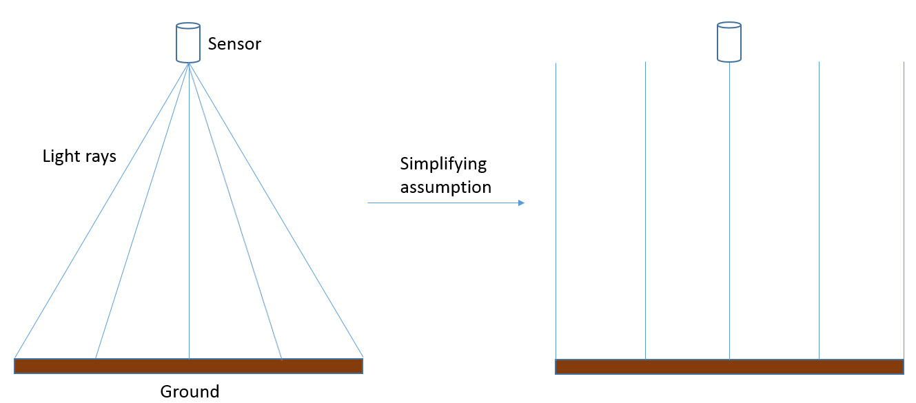
75: In reality, an image is created from light reaching the sensor at different angles from different parts of the Earth’s surface. For present purposes, we can assume that these angles are in fact not different, and that as a result the distance between the sensor and the Earth’s surface is the same throughout an image. In reality, this assumption is not correct, and scale/spatial resolution actually changes from the image centre toward the edges of the image. Anders Knudby, CC BY 4.0.
This definition of scale is only really relevant for analog aerial photography, where the image product is printed on paper and the relationship between the length of things in the image and the length of those same things in the real world is fixed. For digital aerial photography, or when satellite imagery is used in photogrammetry, the ‘scale’ of the image depends on the zoom level, which the user can vary, so the more relevant measure of spatial detail is the spatial resolution we have already looked at in previous chapters. The spatial resolution is defined as the on-the-ground length of one side of a pixel, and this does not change depending on the zoom level (what changes when you zoom in and out is simply the graininess with which the image appears on your screen). We can, however, define a ‘native’ spatial resolution in a manner similar to what is used for analog imagery, based on the focal length (f), the size of the individual detecting elements on the camera’s sensor (d), and the distance between the sensor and the ground (H):
Single vertical image, hilly terrain
The situation gets more complicated when an image is taken over terrain that cannot reasonably be assumed to be perfectly flat, or when the distance between the sensor and the ground is sufficiently small, or the area covered by the image sufficiently large, that the actual distance between the sensor and the ground changes substantially between different parts of the image:
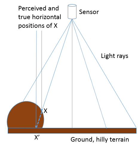
76: When an image is taken closer to the Earth’s surface, or over more hilly terrain, the distance between the sensor and the Earth’s surface cannot be assumed to be constant throughout the image. If not taken into account, this leads to both vertical and horizontal displacement of the imaged objects. Anders Knudby, CC BY 4.0.
Hilly terrain causes a number of problems in photogrammetry, most importantly the vertical and horizontal displacement of imaged objects. As illustrated in Figure 76, if point X is assumed to lie on the flat surface (and not on the hill where it is actually found), based on the imaging geometry its horizontal position will be assumed to be at X’, because that is where the ‘light ray’ intersects the flat ground. In reality, of course, its horizontal position is not at X’. If the surface terrain of the imaged area is known, for example through availability of a high-quality digital elevation model, it can be taken into account when georeferencing the image and the correct intersection between the ‘light ray’ and the ground (on the hill) can be identified. However, if no digital elevation model exists, the effect of terrain – known as relief displacement – cannot be explicitly accounted for, even if it is obvious in the resulting imagery.
Stereo imagery
Until a decade ago, probably the most advanced use of photogrammetry was to use a stereo-pair (two images covering the same area from different points of view) to directly derive a digital elevation model from the imagery, which also enabled things like measuring the heights of things like buildings, trees, cars, and so on. The basic principle of stereoscopy, as the technique is called, is a replication of what you do with your two eyes all the time – by viewing an object or a landscape from two different angles it is possible to reconstruct a three-dimensional model of it. While there is a sophisticated art to doing this with high accuracy (an art we cannot explore as part of this course), we will review the basic idea here.
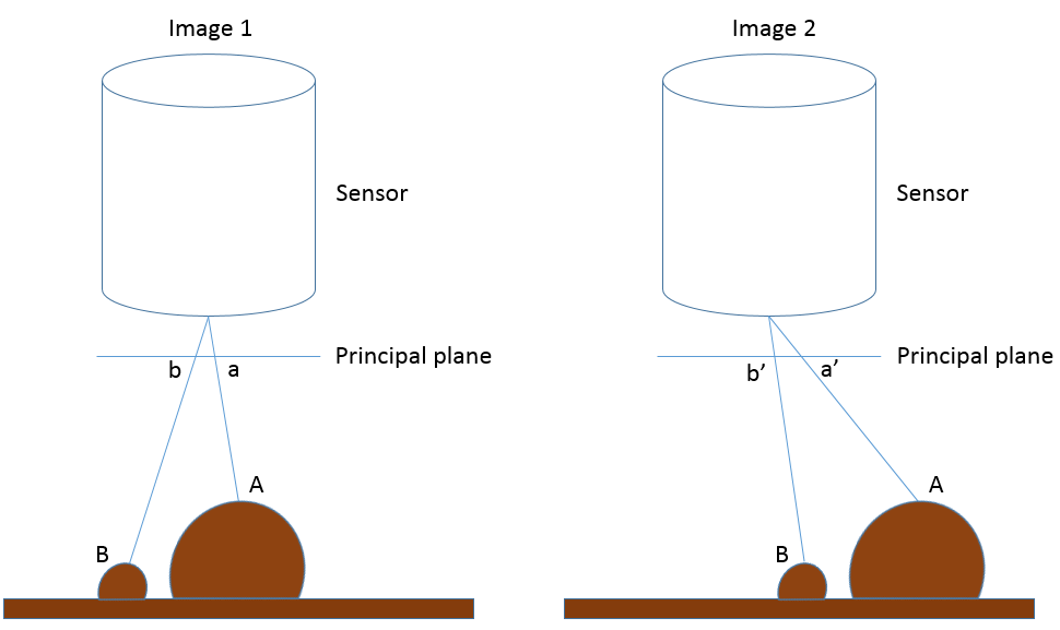
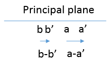
77: Illustration of how the apparent horizontal positions of point A and B change between the two images that form a stereo view of the area. Sensor size has been greatly exaggerated to show the location of each point on the principal plane. Anders Knudby, CC BY 4.0.
In Figure 77, Image 1 and Image 2 represent a stereo view of the landscape that contains some flat terrain and two hills, with points A and B. On the left side of the figure (Image 1), a and b denote the locations each point would be recorded at on the principal plane in that image, which corresponds to where the points would be in the resulting image. On the right side of the figure, the camera has moved to the left (following the airplane’s flight path or the satellite’s movement in its orbit), and again b’ and a’ denote the locations each point would be recorded at on the principal plane in that image. The important thing to note is that a is different from a’ because the sensor has moved between the two images, and similarly b is different from b’. More specifically, as illustrated in Figure 78, the distance between a and a’ is greater than the distance between b and b’, because A is closer to the sensor than B is. These distances, known as parallax, are what convey information about the distance between the sensor and each point, and thus about the altitude at which each point is located. Actually deriving the height of A relative to the flat ground level or relative sea level or a vertical datum, or even better deriving a digital elevation model for the entire area, requires careful relative positioning of the two images (typically done by locating lots of surface features that can be recognized in both images) as well as knowing something about the position and orientation of the sensor when the two images were acquired (typically done with GPS-based information), and finally knowing something about the internal geometry of the sensor (typically this information is provided by the manufacturer of the sensor).
The math applied in stereoscopy is fairly complicated, but in practice even a novice can produce useful digital elevation models from stereo imagery with commercial software. While some specialized photogrammetry software exists, the large commercial remote sensing software packages typically include a ‘photogrammetry module’ that can help you produce digital elevation models even if you are not an expert photogrammetrist. In the above, we have assumed nadir-looking imagery (i.e. that the sensor was pointed straight toward Earth for each image) because the concepts get more complicated when this is not the case, but mathematical solutions exist for oblique imagery as well. In fact, one of the useful attributes of several modern satellites carrying imaging sensors is their ability to tilt, which allows two images to be captured by the same sensor during the same orbit. As the satellite approaches its target, it can be pointed forward to capture an image, and later in the orbit it can be pointed backward to image the same area again from a different angle.
Structure-from-Motion (multi-image photogrammetry)
As it happens occasionally in the field of remote sensing, techniques developed initially for other purposes (for example medical imaging, machine learning, and computer vision) show potential for processing of remote sensing imagery, and occasionally they end up revolutionizing part of the discipline. Such is the case with the technique known as Structure-from-Motion (SfM, yes the ‘f’ is meant to be lower-case), the development of which was influenced by photogrammetry but was largely based in the computer vision/artificial intelligence community. The basic idea in SfM can be explained with another human vision parallel – if stereoscopy mimics your eye-brain system’s ability to use two views of an area acquired from different angles to derive 3D information about it, SfM mimics your ability to close one eye and run around an area, deriving 3D information about it as you move (don’t try this in the classroom, just imagine how it might actually work!). In other words, SfM is able to reconstruct a 3D model of an area based on multiple overlapping images taken with the same camera from different angles (or with different cameras actually, but that gets more complicated and is rarely relevant to remote sensing applications).
There are a couple of reasons why SfM has quickly revolutionized the field of photogrammetry, to the point where traditional stereoscopy may quickly become a thing of the past. Some of the important differences between the two are listed below:
- Traditional (two-image) stereoscopy requires that the internal geometry of the camera is characterized well. While there are established processes for figuring out what this geometry is, they require a moderate level of expertise and require the user to actually go through and ‘calibrate’ the camera. SfM does this camera calibration using the very same images that are used to map the area of interest.
- In a similar vein, traditional stereoscopy requires that the position and orientation (pointing) of the camera is known with great precision for each image. SfM benefits from approximate information on some or all of those parameters, but does not strictly need them and is able to derive them very accurately from the images themselves. Because many modern cameras (like the ones in your phone) have internal GPS receivers that provide approximate location information, this allows consumer-grade cameras to be used to derive remarkably accurate digital elevation models.
- For both techniques, if the camera positions are not known, the 3D model reconstructed from the images can be georeferenced using imaged points of known location. In this way the two techniques are similar.
- The rapid evolution of drones has provided average people with a platform to move a consumer-grade camera around in ways that were previously limited to people with access to manned aircraft. Images taken by drone-based consumer-grade cameras are exactly the kind of input necessary in an SfM workflow, while they do not work well in the traditional stereoscopy workflow.
As mentioned above, SfM uses multiple overlapping photos to produce a 3D model of the area imaged in the photos. This is done in a series of steps as outlined below and shown in Figure 79:
Step 1) Identify the same features in multiple images. To be able to identify the same features in photos taken from different angles, from different distances, with the cameras not always being oriented in the same way, possibly even under different illumination conditions, in extreme cases even with different cameras, SfM starts by identifying features using the SIFT algorithm. These features are typically those that stand out from their surroundings, such as corners or edges, or objects that are darker or brighter than their surroundings. While many such features are easy to identify for humans, and others are not, the SIFT algorithm is specifically designed to allow the same features to be identified despite the challenges circumstances outlined above. This allows it to work especially well in the SfM context.
Step 2) Use these features to derive interior and exterior camera information as well as 3D positions of the features. Once multiple features have been identified in multiple overlapping images, a set of equations are solved to minimize the overall relative positional error of the points in all images. For example, consider the following three (or more) images, in which the same multiple points have been identified (shown as coloured dots):
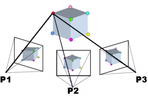
79: Example of bundle block adjustment in SfM. Sfm1 by Maiteng, Wikimedia Commons, CC BY-SA 4.0.
Knowing that the red point in P1 is the same as the red point in P2 and P3 and any other cameras involved, and similarly for the other points, the relative position of both the points and the camera locations and orientations can be derived (as well as the optical parameters involved in the image-forming process of the camera). (Note that the term ‘camera’ as used here is identical to ‘image’).
The initial result of this process is a relative location of all points and cameras – in other words the algorithm defined the location of each feature and camera in an arbitrary three-dimensional coordinate system. Two pieces of additional information can be used to transform the coordinates from this arbitrary system to real-world coordinates like latitude and longitude.
If the geolocation of each camera is known prior to this process, for example if the camera produced geotagged images, the locations of the cameras in the arbitrary coordinate system can be compared to their real locations in the real world, and a coordinate transformation can be defined and also applied to the locations of the identified features. Alternatively, if the locations of some of the identified features is known (e.g. from GPS measurements in the field), a similar coordinate transformation can be used. For remote sensing purposes, one of these two sources of real-world geolocation information is necessary for the resulting product to be useful.
Step 3) Based on the now geo-located features, identify more features in multiple images, and reconstruct their 3D position. Imagine that there is a little grey dot close to the red point in Figure 79, say ¼ of the way toward the green point, in that direction (there isn’t, which is why you need to imagine it!). This little grey dot was too faint to be used as a SIFT feature, and so was not used to derive the initial location of features and orientations of cameras. However, now that we know where to find the red dot in each image, and we know the relative position of each of the other dots, we can estimate where this grey dot should be found in each of the images. Based on this estimate, we might actually be able to find the grey dot in each image, and thus estimate its location in space. Once identified and located in space, we can also assign a colour to the point, based on its colour in each of the images it was found in. Doing this for millions of features found in the complete set of images is called point cloud densification, and is an optional but almost universally adopted step in SfM. In areas with sufficient difference between the colours of neighbouring pixels in the relevant images, this step can often lead to the derivation of the location of each individual pixel in a small area of an image. The result of this step therefore is an incredibly dense ‘point cloud’, in which millions of point are located in the real world. An example is shown below:
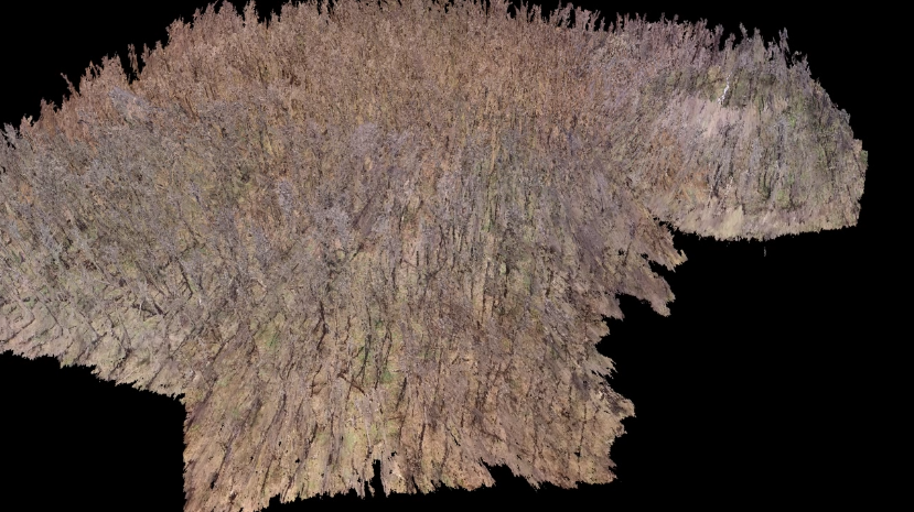
80: Example of dense point cloud, created for a part of Gatineau Park using drone imagery. Anders Knudby, CC BY 4.0.
Step 4) Optionally, use all these 3D-positioned features to produce an orthomosaic, a digital elevation model, or other useful product. The dense point cloud can be used for a number of different purposes – some of the more commonly used is to create an orthomosaic and a digital elevation model. An orthomosaic is a type of raster data, in which the area is divided up into cells (pixels) and the colour in each cell is what it would look like if that cell was viewed directly from above. An orthomosaic is thus similar to a map except that it contains information on surface colour, and represents what the area would look like in an image taken from infinitely far away (but with very good spatial resolution). Orthomosaics are often used on their own because they give people a quick visual impression of an area, and they also form the basis for map-making through digitization, classification, and other approaches. In addition, because the elevation is known for each point in the point cloud, the elevation of each cell can be identified in order to create a digital elevation model. Different algorithms can be used to do this, for example identifying the lowest point in each cell to create a ‘bare-earth’ digital terrain model, or by identifying the highest point in each cell to create a digital surface model. Even more advanced products can be made, for example subtracting the bare-earth model from the surface model to derive estimates of things like tree and building height.
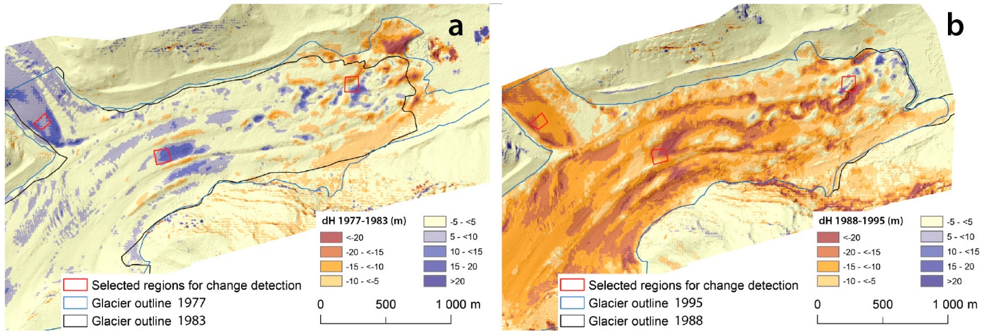
Change detection with photogrammetry
While the creation of digital elevation models or other products using stereoscopy or Structure-from-Motion approaches can be useful on its own, an increasingly common application of these techniques is for surface change detection. If, for example, a digital elevation model is created for a glacier one year, and a new one created two years later, changes in the shape of the glacier’s surface can be mapped with great precision. Landslides, thaw slumps, vegetation change, snow depth changes throughout a season – many changes in the physical environment can be detected and quantified by measuring changes in the horizontal or vertical position or the Earth’s surface. Given the relatively recent development of SfM technology, and the still-developing capabilities and cost of camera-equipped drones, this is a rapidly developing field likely to be useful in surprising and unsuspected parts of the remote sensing field. Figure 81 illustrates this principle comparing the outline and of the glacier and changes in surface elevation at two different times.