1.15: Lab 15 - Fluvial Geomorphology

Learning Objectives

• Explain the relationship between streamflow and carrying capacity.
• Interpret a hydrograph and compare rural and urban hydrographs.
• Analyze a stream profile to determine how flow rates influence erosion and deposition.
• Calculate stream discharge.
• Identify the processes that create meandering streams, oxbow lakes, and waterfalls.
• Compare and contrast three deltas.
• Analyze fluvial processes on topographic maps before and after dam removals.

Introduction

Fluvial processes refer to processes related to rivers and streams and the landforms created by them. Due to the circulating effects of the hydrologic cycle, nearly every landscape is influenced by impacts of water flowing over the surface. Even in our desert regions, where precipitation is rare, we still see dried riverbeds (arroyos) and catchment basins (playas). Rivers have the ability to erode a landscape, transport material to other areas, and form other landscape features by depositing the materials in other locations.

In this lab you will learn about the factors and processes that influence the erosion, transportation, and deposition of material by water. You will also investigate the formation of landscape features that are created by rivers.

Part A. Streamflow and Carrying Capacity

Stream capacity refers to the total sediment that a stream carries. Stream competence is the ability of a stream to transport a particular size particle. Both of these variables change with the stream’s velocity. Streams and rivers transport materials in a number of different ways. These include dissolved load, suspended load, and bed load:

➢ Dissolved load is composed of ions in solution. These ions are usually carried in the water all the way to the ocean.

➢ Suspended load is composed of sediments carried as solids in water. The size of particles that can be carried is determined by the stream’s velocity. Faster streams can carry larger particles. Streams that carry larger particles have greater competence. Streams with a steep gradient (slope) have a faster velocity and greater competence, as well.

➢ Bed load are sediments that are too large to be carried as suspended load; these sediments are bumped and pushed along the stream bed. Bed load sediments do not move continuously: smaller particles are temporarily lifted and then dropped again. This jumping process is referred to as saltation. The intermittent movement of pushing, shoving, and dragging is called traction. Streams with high velocities and steep gradients do a great deal of down-cutting into the stream bed, which is primarily accomplished by movement of particles that make up the bed load.^[263]

Exercise \(\PageIndex{1}\)

1. In the space below, sketch and label a cross-section of a river with dissolved, suspended, and bed load. Include both the saltation and traction processes.

One of the strongest factors affecting a stream’s ability to erode and transport material is the flow speed of the water. A Swedish geographer, Filip Hjulström, ran a series of experiments on the ability of water to transport specific particle sizes. Based on his research, he developed the Hjulström curve (Figure 15.1). The diagram shows the size of the particles that flowing water can erode and transport, compared to the speed of the water. Clay-sized grains are less than 0.002 millimeters (mm) in size, silt-sized grains are between 0.002mm to 0.05mm, and sand-sized grains are from 0.05mm to 2mm in size. Note that on Figure 15.1 the x-axis shows the grain sizes in millimeters and the y-axis shows the flow speed of the river in centimeters per second (cm/s).

There are several factors that influence the flow speed of the water. These include the amount of water, the slope of the stream bed, and the shape of the channel. You will explore some of these factors throughout this lab.

Figure 15.1: Hjulström Curve. Figure by Scott Crosier is licensed under CC BY-NC-SA 4.0

Exercise \(\PageIndex{2}\)

2. Refer to Figure 15.1.

1. What is the minimum speed of water that will erode clay particles?

2. What is the minimum speed of water that will erode sand particles?

3. Why do you think the speeds to erode clay and sand particles are different? Explain your response in one sentence.

4. You are exploring a creek bed and come upon a rock which has been transported downstream. The rock is the size of a bowling ball (8½ inches; 215 millimeters). How fast must the water have been moving to transport that rock?

5. You are studying a river that is flowing at 1 meter/second (there are 100 centimeters in 1 meter). What size materials would you expect to see...

1. ...eroding?

2. ...being transported?

3. ...being deposited on the riverbed?

Hydrographs and Storm Events

One of the factors that influences the speed of water in a channel is the amount of water. During a storm event, the amount of water being forced through a channel can be significant. One way of understanding the behavior of water in a channel during a storm event is by creating a hydrograph. Figure 15.2 illustrates two hypothetical hydrographs, one line representing a hydrograph for a rain event in an urbanized area and another line representing a hydrograph for the same rain event, but in a rural area.

The hydrograph illustrates the rate of flow as a result of the rain event in two different hypothetical situations: as it would be in an urban area and how it would look in a rural area. Regardless of the setting, you will notice on the hydrographs that although the rain event illustrated lasted from 14:00 (2 p.m.) until 21:00 (9 p.m.) the peak flow at the hypothetical stream gauges did not take place until some time later. To explain this, consider what is happening. Rain falls on the ground, some water begins to pool, and eventually the water runs into rills and gullies, to eventually join the stream.

Stream flow, or discharge, is the volume of water that moves over a particular point of a stream at a particular point in time. The duration of time between the peak rainfall and the peak discharge is referred to as the lag time. You will notice that the lag time for urbanized areas and rural areas is different. In some very large drainage systems (such as the Mississippi River), this lag time can be even greater. In strong storm events, the discharge can also stay elevated for a greater duration. Spring melt-off of snow can also contribute to an increase in discharge.

Figure 15.2: Two Hypothetical Hydrographs for Rural and Urban Environments. Figure by Scott Crosier is licensed under CC BY-NC-SA 4.0

Exercise \(\PageIndex{3}\)

3. Refer to Figure 15.2.

1. What is the approximate lag time for the urbanized area?

2. What is the approximate lag time for the rural area?

3. Use Your Critical Thinking Skills: Why is there a difference between the lag time for an urbanized area and a rural area? Explain your response in one to two sentences.

4. Use Your Critical Thinking Skills: What if the storm event dropped snow rather than rain? What would the hydrograph look like? Explain your response in one to two sentences.

5. Use Your Critical Thinking Skills: What if the storm event was a warmer, more tropical storm dropping a larger quantity of warm rain on a pre-existing snow pack? What would the hydrograph potentially look like? Explain your response in one to two sentences.

Check It Out! More About America’s Rivers

Interested in further exploring the flows of America’s rivers? The US Geological Survey has made some of that information available online. Check out Water Watch to see current streamflow data, locations experiencing drought, and locations experiencing floods.

Part B. Stream Profiles

In addition to looking at the water flowing through rivers, we also study rivers by looking at the slope and the shape of rivers. These plots are referred to as stream profiles. A longitudinal profile illustrates the elevation compared to the mouth of a river (Figure 15.3). Vertical profiles illustrate a cross-cut view of a river at a specific location. It shows the water level, the topography under the river, and the surrounding floodplain (Figure 15.4). Floodplains are relatively flat, low-lying areas located near the mouth of a river that are prone to flooding during periods of high discharge.

Longitudinal Profiles

Figure 15.3 shows a hypothetical longitudinal river profile. It is, in essence, a graph showing the elevation of the river as it moves from the mountains or hills where it begins (its head) and how that elevation changes as it approaches the lake or ocean it enters (its mouth).

Figure 15.3: Hypothetical Longitudinal River Profile. Figure by Scott Crosier is licensed under CC BY-NC-SA 4.0

Exercise \(\PageIndex{4}\)

4. On Figure 15.3, above, label where you observe a steeper slope and a gentler slope.

With different slopes, you will see different speeds of water flow. As you learned in the previous section of this lab, different speeds of water are directly related to erosion. Thus, river erosion is not the same through the entire course of a river.

5. In what part of the river would you expect to see the greatest amount of erosion taking place? Explain your response in one sentence. Be sure to consider the river’s gradient and velocity.

6. Where would you expect to see deposition of sediment? Explain your response in one sentence. Be sure to consider the river’s gradient and velocity.

7. What happens to transported materials in a river, once the river reaches the mouth (flowing into a lake or ocean) and the movement stops? What type of feature is created? Explain your response in two to three sentences. Hint: consider what feature is found at the mouth of most major rivers throughout the world.

Vertical Profiles

Another way of looking at a river is in a vertical profile. Although it does not illustrate the movement of water through the entire course of the river, it does provide a clear snapshot at one specific location of the river. As illustrated in Figure 15.4, a vertical profile shows the cross-cut view of the river. It illustrates the riverbed shape, the area where water flows (the active channel) and often will illustrate the floodplain found on both sides of the river. These vertical profiles are developed through basic survey work, measuring the depth at regular intervals, perpendicular to the stream flow.

Figure 15.4: Hypothetical Vertical River Profile. Figure by Scott Crosier is licensed under CC BY-NC-SA 4.0

Calculating Stream Discharge

Hydrologists—scientists who study the effects of water on and near the surface of the Earth—survey and create stream profiles to better understand the erosional impacts of a river as well as measuring the amount of water flowing through a specific area of a river. This is referred to as the stream discharge. In Figure 15.4, above, let us assume that the active channel has an area of 4.25 square meters (m²) and that the average flow rate of the river is 1.4 meters per second (m/sec). Figure 15.5 diagrams one of these two variables: the area of an active channel.

Figure 15.5: Volume of Water Passing through the River. Figure by Scott Crosier is licensed under CC BY-NC-SA 4.0

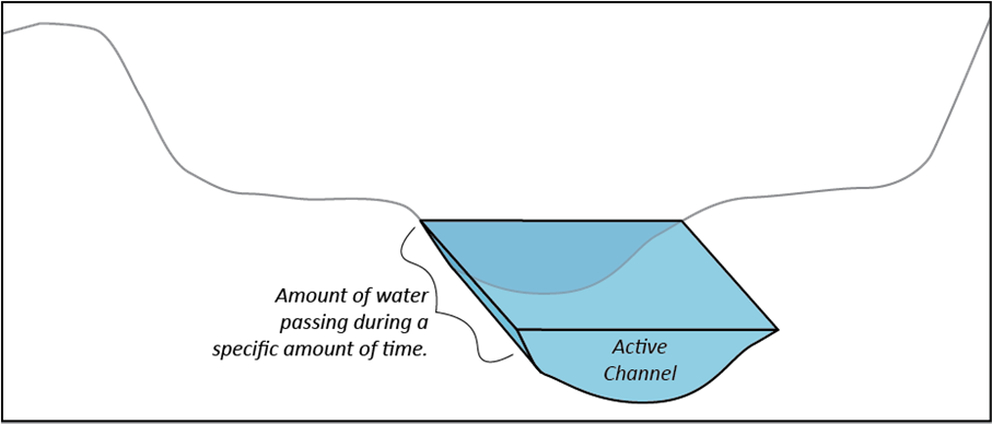
To calculate the stream discharge, multiply the active channel by the flow rate. For reference, one cubic meter (m³) has a volume of 1,000 liters, which is equivalent to about 264 gallons.

Area of Active Channel x Velocity = Stream Discharge

4.5 m² x 1.4 m/sec = 6.3 m³/sec

Exercise \(\PageIndex{5}\)

8. Now you try! Assume you and some classmates have surveyed a stream and found the active channel to be 7.6 meters squared. The average flow rate is 0.75 meters per second.

1. How many cubic meters of water are passing that location per second? Show your calculation.

2. How much water is passing that location per minute? Show your calculation.

The USGS operates over 8,200 continuous-record streamgages that provide streamflow information for a wide variety of uses including flood prediction, water management and allocation, engineering design, research, operation of locks and dams, and recreational safety and enjoyment.^[269] Between April 29 and May 1, 2017, a vigorous weather system delivered intense rain, heavy snow, and tornadoes across the central and southern United States. In many areas, rainfall totals surpassed 9 inches (23 centimeters). This deluge led to dangerous flash floods and rivers cresting at record and near-record heights.^[270] The discharge data collected at three streamgages along the Mississippi River during this May 2017 flood event are shown in Figure 15.6. The streamgage data for the point most upstream on the river is shown in red (St. Louis, Missouri, located at approximately 39°N latitude). The streamgage data for Memphis, Tennessee, located at approximately 35°N latitude, is shown in green. The streamgage data for the point most downstream on the river is shown in blue (New Orleans, Louisiana, located at approximately 30°N latitude).

Figure 15.6: Hydrograph for Three Locations along the Mississippi River during a May 2017 Flood Event. Figure adapted from the USGS National Water Information System

Exercise \(\PageIndex{6}\)

9. Refer to Figure 15.6.

1. Apply What You Learned: Review the daily discharge data prior to the storm event (April 28 and earlier). Why might the daily discharge for the Mississippi River at St. Louis be much lower than the daily discharge for the Mississippi River at Memphis or New Orleans? Explain your response in one to two sentences.

2. On the graph, lightly shade the dates when the storm precipitation was the heaviest (April 29 and May 1).

3. Describe the daily discharge curves (the lines on the graph) for each location from April 29 through May 15, 2017.
   1. St. Louis:
   2. Memphis:
   3. New Orleans:

4. Apply What You Learned: What is the lag time for each location?
   1. St. Louis:
   2. Memphis:
   3. New Orleans:

5. Compare the daily discharge of the Mississippi River at St. Louis from April 24 to May 6, 2017. How much did the daily discharge increase during these dates?

6. Use Your Critical Thinking Skills: Why do you think the daily discharge for St. Louis increased and decreased more rapidly than the daily discharge for Memphis or New Orleans? Explain your response in one to two sentences.

Check It Out! National Water Information System Mapper

Is there a streamgage near you? Check out the National Water Information System Mapper to find the locations of streamgages and access discharge data.

Floodplains

You will also notice in Figure 15.4 (shown earlier in the lab) that on both sides of the river is a region referred to as a floodplain. As the name implies, these floodplains are the areas where water flows when the water level rises higher than normal. In some stream channels, these floodplains and banks are easy to identify. In other areas, such as the Sacramento Valley, these floodplains are very wide. These floodplains are often rich agricultural soils, replenished each flood season with new, nutrient-rich sediments. The wealth and prosperity of Ancient Egypt was due to the nutrient-rich sediments flooding down the Nile River each year. Often when significant storm events take place, individuals who have used the floodplain for a variety of reasons are taken by surprise, at times with devastating outcomes.

Check It Out! More About Floodplains

Do you live on or near a floodplain? Find out! The Federal Emergency Management Agency (FEMA) has mapped out all of the floodplains. Go to the FEMA Flood Map Service and search for your address.

Exercise \(\PageIndex{7}\)

10. Use Your Critical Thinking Skills: Now you’re the city planner! The Federal Emergency Management Agency (FEMA) has designated a region near your community as a 100-year floodplain. This designation suggests that the region, statistically, has a 1% of a flood of a given magnitude in any given year. (Hint: A 100-year floodplain can be interpreted as a 1 in 100 chance).

1. As a city planner, what do you believe is an appropriate use of that land? What is not? Explain your response in three to four sentences.

2. A land owner proposed building a house in the floodplain. Do you approve the building permits? What extra requirements might you require for the building? Explain your response in two to three sentences.

3. What criteria do you use in these decisions? List at least three criteria.

Part C. Rivers Shaping the Landscape

There are a variety of features that are created as a result of river action. Some are formed through erosional processes. Others are created as a result of deposition. Some are formed by a combination of the two processes.

Meandering Streams

One such feature that results from both erosion and deposition is a meandering stream. Once a river descends down to a lower valley floor, the flow rates of the water tend to vary within the active channel. On straight stretches of river, the flow rate is typically slower along the bed due to friction on the surface. However, whenever a slight bend or turn takes place, the flow rates on either side of a river are different as illustrated in Figure 15.7. Earlier in this lab you learned the impacts of water speed on the erosional and depositional capacity of a river. Figure 15.7 shows that water speed in the river varies depending on the shape of the river channel.

Figure 15.7: The Velocity of a Stream depends on whether the Channel is Straight or Curved. Figure by Steven Earle is licensed by CC BY 4.0

Exercise \(\PageIndex{8}\)

11. Refer to the river channel labeled B in Figure 15.7.

1. On which side of the river would you anticipate more erosion? On the outside of the turn (right side in diagram example B) or the inside (on the left side in diagram example B)?

2. On which side of the river shown on example B would you anticipate more deposition?

3. Apply What You Learned: If this were to occur over a great deal of time, what change would you anticipate for the path of the river? Explain your response in one to two sentences.

This idea of uneven erosion and deposition of either side of a river channel is exactly what creates a meandering stream. Figure 15.8 illustrates the speed of water in a channel as it responds to turns in the course of the river. The red arrows illustrate the faster moving water.

Figure 15.8: Pathway of Fastest Water Flow in a Meandering Stream. Figure by Scott Crosier is licensed under CC BY-NC-SA 4.0

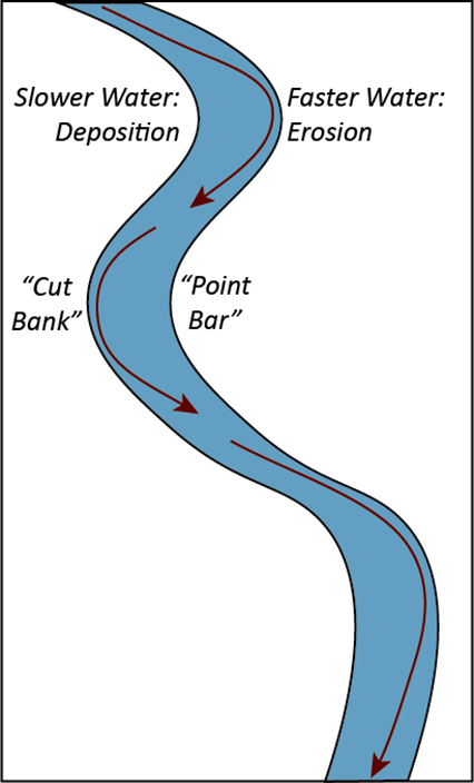
As a river turns, the outside of the turn is referred to as the cut bank. It is the region with the greatest amount of erosion. On the inside of the turn, water flows more slowly,resulting in deposited material. This is called the point bar.

Exercise \(\PageIndex{9}\)

12. On the river channel labeled B in Figure 15.7, label the cut bank and the point bar. Also, label the cut bank and point bar on the bird’s-eye view of the river shown on the left-side of Figure 15.7.

Oxbow Lakes

At times, the river cuts through and part of a turning loop is cut off from the course of the river. Although the old channel is still there, the water flow does not use that channel. The slower movement on both ends of the cut off section promotes sediment deposits and eventually the old channel is completely cut off of the river and forms a curved lake. This is referred to as an oxbow lake. Figure 15.9 shows how the progression of a meandering river creates an oxbow lake over time. In this diagram, the far-left diagram (labeled A) represents the oldest time period and the far-right diagram (labeled D) represents the most recent time period.

Figure 15.9: Progression of a Meandering Stream. Figures by Scott Crosier are licensed under CC BY-NC-SA 4.0

Exercise \(\PageIndex{10}\)

Virtual Field Trip to a Meandering River

13. Using Google Maps or Google Earth, navigate to the following coordinate along the Sacramento River in Butte County, California: 39.67, -121.97. Turn on the satellite view. Zoom out to an extent where you can see several of the bends in the river.
14. In the box provided below (Figure 15.10), sketch the pathway of the Sacramento River where the river is flowing in from the upper right (Northeast) corner, making a significant turn on the left (West) side, and eventually flowing out the bottom (South) of the box.

Figure 15.10: Blank Map.

15. In your sketch above (Figure 15.10), label the cut banks and point bars.

16. Do you see any signs that suggest there is or was an oxbow lake present? Sketch where you suspect and label it on Figure 15.10.

17. Based on what you have learned regarding the migration patterns of rivers, where might you anticipate a future oxbow lake? Outline with a dotted line and label the area on Figure 15.10.

Waterfalls

In previous labs, you have explored different aspects of rock structures. When a river is flowing over different types of rock, the ability of the river to erode the rock will vary. Some rock is very hard and resistant to erosion while other layers may be softer and more prone to erode. Many waterfalls occur at the boundary of these layers. Water flowing over the harder rock may have very little erosional impact. But, once it begins flowing over the softer rock, the water is able to erode and transport that material away. This develops a step in the river channel leading to faster movement of water, which leads to increased erosion and transportation as illustrated in Figure 15.11.

Figure 15.11: Development of a Waterfall. Figure by Scott Crosier is licensed under CC BY-NC-SA 4.0

Exercise \(\PageIndex{11}\)

18. Refer to Figure 15.11. Based on what you know about the erosional processes in waterfalls, would you anticipate that the waterfall moves upstream or downstream? Explain your response in one to two sentences.

Deltas

Through this lab you have learned the influence of water movement, specifically in regards to erosion, transportation, and deposition. Faster moving water erodes and transports while slower water causes deposition. But what happens when a river completely stops moving? This occurs when a river reaches a sea or ocean. The material that the river was carrying is deposited, often forming a triangular-shaped extension on the landmass referred to as a delta.

Exercise \(\PageIndex{12}\)

Virtual Field Trip to Three Deltas

19. Perhaps the most iconic of all deltas is where the Nile River flows into the Mediterranean Sea. Using Google Maps or Google Earth, navigate to the following coordinate: 30.81, 31.09. Turn on the satellite view. Zoom out until you can see Cairo to the South and the Mediterranean Sea to the North.

1. Based on the color of the region, what do you suspect in the main land use of the region?

2. What is the overall shape of the area?

3. Zoom further out. What is the land cover for most of the surrounding regions?

20. One of our country’s most iconic waterways is the Mississippi River. The Mississippi flows into the Gulf of Mexico very close to New Orleans. Using Google Maps or Google Earth, navigate to the following coordinate: 29.53, -90.78. To get a full view of the Mississippi River delta, zoom out until you see Biloxi on the east side of the display, Baton Rouge on the north and Lafayette on the west.

1. What is the overall land use for this region?

2. What patterns do you see which are similar to or different from what you saw in Egypt at the River Nile?

3. Use Your Critical Thinking Skills: The Gulf of Mexico is prone to hurricanes and significant storm surges. These are extremely high waves that result from the strong winds in a hurricane. What influence would the Mississippi River delta have on the storm surges? Why might they be important to Gulf Coast cities such as New Orleans? Your response should be two to three sentences in length.

21. Let’s come back to California! The Central Valley has two major rivers (the Sacramento River from the North and the San Joaquin River from the South) that converge further inland. This is due to the coastal range and several bays between the rivers and the Pacific Ocean. This type of delta is unique and is referred to as a “reverse delta” because the sediments are deposited further inland, rather than into the eventual water body such as an ocean. Using Google Maps or Google Earth, navigate to the following coordinate: 38.05, -121.58.

1. As you zoom out, what land use seems to dominate this region?

2. What patterns do you find in common with the other deltas that you have virtually visited?

3. To see the full extent of the delta, zoom out until you see Antioch on the west side of the display and Stockton on the east. In one sentence, describe the patterns of many of the waterways in this region.

22. While you are here, navigate just slightly to the south, to the following coordinate: 37.83, -121.56. This is the beginning of the California Aqueduct! Natural water flow in the southern portion of the central valley is towards the delta. However, at this point, water pulled from the delta region begins its journey south to Southern California. There is a waterway flowing into Clifton Court Forebay from the southeast corner. This is pulling water in from the San Joaquin river much further south near Mendota. On the southwest corner of the Forebay, you will notice the large outlet. This is where the California Aqueduct begins.

1. Using the navigation tools in Google Maps or Google Earth, follow the Aqueduct as far as you can. How far were you able to follow the aqueduct flow?

2. What primary type of landscape does the California Aqueduct flow through?

23. Compare and contrast the Nile, Mississippi, and California deltas. What are the similarities and differences among the deltas? Explain your response in two to three sentences.

Part D. Case Study: Elwha River, Washington

For millennia, the Elwha River ran wild, connecting mountains and seas in a thriving ecosystem. The river proved to be an ideal habitat for anadromous (sea-run) fish, with eleven varieties of salmon and trout spawning in its waters. These fish thrived in the cold, clear waters of the Elwha River and historically served as an important food source for the Lower Elwha Klallam Tribe living along its banks.^[276]

American expansion spurred a continual demand for lumber. The growth of the logging industry in the region brought rapid change to the Olympic Peninsula and specifically to the Elwha River with the construction of two dams. The Elwha and Glines Canyon dams were built in the early 1900s, generating hydropower to supply electricity for the emerging town of Port Angeles and fueling regional growth on the Peninsula. However, construction of the dams blocked the migration of salmon upstream, disrupted the flow of sediment downstream, and flooded the historic homelands and cultural sites of the Lower Elwha Klallam Tribe.¹² Figure 15.12 provides a locator map of the Elwha River in the state of Washington circa 2010.

Figure 15.12: Elwha River Locator Map. Figure by USGS is in the public domain

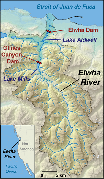
For over a century, the web of ecological and cultural connections in the Elwha Valley were broken—then the river's story changed course. In 1992, Congress passed the Elwha River Ecosystem and Fisheries Restoration Act, authorizing dam removal to restore the altered ecosystem and the native anadromous fisheries therein. After two decades of planning, the largest dam removal in U.S. history began on September 17, 2011. Six months later the Elwha Dam was gone, followed by the Glines Canyon Dam in 2014. Today, the Elwha River once again flows freely from its headwaters in the Olympic Mountains to the Strait of Juan de Fuca.¹²

It was the world’s largest dam-removal project. Over the next five years, water carrying newly freed rocks, sand, silt and old tree trunks reshaped more than 13 miles of river and built a larger delta into the Pacific Ocean. Of the 33 million tons of sediment trapped behind the dams, about 8 million tons resettled along the river or at the mouth, and another 14 million dispersed into the ocean. It would take more than 70 dump trucks running 24 hours a day for five years to move that much dirt and debris downstream. Piled up, the sediment would form a cone about one-third of a mile in diameter and taller than a 50-story building (Figure 15.13).^[278]

Figure 15.13: Size Comparison of Elwha River Sediment. Figure by USGS is in the public domain

Figure 15.14 shows the Elwha River delta after dam removal. Notice the brown sediment flowing into the darker colored water of the Strait of Juan de Fuca.

Figure 15.14: Elwha River Delta after Dam Removal. Figure by Jeff Duda, USGS is in the public domain

Let’s use topographic maps to explore the fluvial geomorphology of the Elwha River before and after dam removal.

If you need a quick review of topographic maps, check out the Topographic Map Symbols document from the USGS.

Step 1

Go to the file in the google drive folder to access the topographic map from 1950 (before the dams were removed).

Step 2

Use the plus (+) sign and minus (-) sign to zoom in and out of the map, as needed. When zoomed in, you can click and drag your mouse pointer to view different portions of the map.

Step 3

Locate the Elwha River, the Upper Elwha Dam, and the Olympic Power Plant, which is at the site of the Elwha Dam. Note that the Upper Elwha Dam is also known as the Glines Canyon Dam.

Exercise \(\PageIndex{12}\)

23. Does the Elwha River flow to the north or to the south? How can you tell?

24. Where do you find evidence that the Elwha River has changed its course over time?

25. Calculate the gradient of the Elwha River between the Upper Elwha Dam and the Olympic Power Plant.

1. Use the graphic scale at the bottom of the topographic map to find the distance between the Upper Elwha Dam and the Olympic Power Plant. What is the estimated distance in miles?

2. Find the contour line at the Upper Elwha Dam. What is the dam’s elevation?

3. Find the contour line at the Olympic Power Plant. What is the power plant’s elevation?

4. What is the difference in elevation (in feet) between these two locations? Show your work.

5. Divide the difference in elevation by the distance between the two locations. Show your work. Your answer should be in feet per mile.

Step 4

Go to the file in the google drive folder to access the topographic map from 2020 (after the dams were removed). Note: this is a very large file and may take a few moments to load.

Step 5

Use the plus (+) sign and minus (-) sign to zoom in and out of the map, as needed. When zoomed in, you can click and drag your mouse pointer to view different portions of the map.

Exercise \(\PageIndex{13}\)

26. Where does the Elwha River have the steepest channel? At this location, what is the difference in elevation from the riverbank to the top of the cliff at the side of the river?

Step 6

Keep both maps open in different tabs in order to compare the Elwha River between 1950 and 2020. Refer to the selected topographic map symbols shown in Appendix 15.1.

Exercise \(\PageIndex{14}\)

27. What are three major differences along the Elwha River that you notice between the 1950 and 2020 topographic maps?

Step 7

Search the internet to find out about any dams, dam construction/maintenance projects, and dam removal projects in the county where you live.

Exercise \(\PageIndex{15}\)

28. Would you tend to support the construction of new dams in your county? Explain your response in two to three sentences.

Part E. Wrap-Up

Consult with your geography lab instructor to find out which of the following wrap-up questions you should complete. Attach additional pages to answer the questions as needed.

Exercise \(\PageIndex{16}\)

29. What is the most important idea that you learned in this lab? In two to three sentences, explain the concept and why it is important to know.

30. What was the most challenging part of this lab? In two to three sentences, explain why it was challenging. If nothing challenged you in the lab, write about what you think challenged your classmates.

31. What is one question that you have about what you learned in this lab? Write your question along with one to two sentences explaining why you think your question is important to ask.

32. Review the learning objectives on page 1 of this lab. How would you rate your understanding or ability for each learning objective? Write one sentence that addresses each learning objective.

33. Sketch a concept map that includes the key ideas from this lab. Include at least five of the terms shown in bold-faced type.

34. Create an advertisement to educate your peers on the important information that you learned in this lab. Include at least three key terms in your advertisement. The advertisement should be about half a page in size (about 4 inches by 6 inches).

35. One way to think of physical geography is that it is the study of the relationships among variables that impact the Earth's surface. Select two variables discussed in this lab and describe how they are related.

36. How does what you learned in this lab relate to your everyday life? In two to three sentences, explain a concept that you learned in this lab and how it relates to your day-to-day actions.

37. How does what you learned in this lab relate to current events?
    1. Write the title, source, and date of a news item that relates to this lab.
    2. In two to three sentences, discuss how the news item relates to what you have learned in this lab.
    3. In one to two sentences, discuss whether or not the news item accurately represents the science that you learned. Tip: consider whether or not the news item includes the complexity of the topic.

38. Search O*NET OnLine to find an occupation that is relevant to the topics presented in today's lab. Your lab instructor may provide you with possible keywords to type in the Occupation Quick Search field on the O*NET website.
    1. What is the name of the occupation that you found?
    2. Write two to three sentences that summarize the most important information that you learned about this occupation.
    3. What is one question that you would want to ask a person with this occupation?

Appendix 15.1: Selected Topographic Map Symbols

Excerpts from USGS

---

^[263] Water Erosion and Deposition by CK-12 is licensed under CC BY-NC 4.0

^[269] Text by USGS is in the public domain

^[270] Text by NASA’s Earth Observatory

^[276] Text by National Park Service is in the public domain

^[278] Text by USGS is in the public domain