8.3: Ekman Motion

During his Arctic expedition in the 1890s, Fridtjof Nansen noticed that drifting ice moved in a direction about 20° to 40° to the right of the wind direction. The deflection occurs because water set in motion by the wind is subject to the Coriolis effect (CC12). The surface current that carries drifting ice does not flow in the direction of the wind but is deflected cum sole (“with the sun”), in the same way we see the sun move across the sky—to the right in the Northern Hemisphere and to the left in the Southern Hemisphere (CC12). Remember the term cum sole. It always means “to the right in the Northern Hemisphere and to the left in the Southern Hemisphere.”

The Ekman Spiral

As surface water is set in motion by the wind, it successively sets in motion a series of thin layers of water (Fig. 8-2a), transferring energy down into the water column. The surface layer is driven by the wind and deflected by the Coriolis Effect. Each successively lower layer is driven by the layer above, with speed decreasing in each lower layer, and each layer is also deflected by the Coriolis effect. When it is set in motion by friction with the layer above, each layer’s direction of motion is deflected by the Coriolis effect cum sole to the direction of the overlying layer. This deflection establishes the Ekman spiral (Fig. 8-4), named for the physicist who developed the mathematical relationships to explain Nansen’s observations that floating ice does not follow the wind direction.

Surface water set in motion by the wind is deflected at an angle cum sole to the wind (Fig. 8-4). Ekman’s theory predicts this angle to be 45° cum sole to the wind direction under ideal conditions, with constant winds and a water column of uniform density. Under normal conditions, the deflection is usually less. As depth increases, current speed is reduced, and the deflection increases. The Ekman spiral can extend to depths of 100 to 200 m, below which the energy transferred downward from layer to layer becomes insufficient to set the water in motion. This depth is a little greater than the depth where the flow is opposite to the surface current direction. This depth is called the “depth of frictional influence.” At this depth, the current speed is about 4% of the surface current speed. The water column above the depth of frictional influence is known as the “wind-driven layer.”

Figure 8-4. The Ekman spiral. (a) In the Northern Hemisphere, the Coriolis deflection causes a surface current to flow at an angle to the right of the wind direction. As the kinetic energy of the wind-driven current is transferred downward in the water column, each layer of water is deflected to the right of the direction of the layer above, producing a spiraling current called the Ekman spiral, in which speed decreases with depth. (b) If the wind blows long enough over deep water, the Ekman spiral motion becomes fully developed. When the spiral is fully developed in the Northern Hemisphere, the surface current direction is 45° to the right of the wind direction, and the net water transport is 90° to the right of the wind direction. In the Southern Hemisphere, the deflection and net water transport are to the left.

The most important feature of the Ekman spiral is that water in the wind-driven layer is transported at an angle cum sole to the wind direction and that the deflection increases with depth. Ekman showed that, under ideal conditions, the mean movement of water summed over all depths within the wind-driven layer is at 90° cum sole to the wind. Such movement is called Ekman transport.

For the Ekman spiral to be fully established, the water column above the depth of frictional influence must be uniform or nearly uniform in density, water depth must be greater than the depth of frictional influence, and winds must blow at a constant speed for as long as a day or two. Because these conditions are rare, the Ekman spiral is seldom fully established.

Pycnocline and Seafloor Interruption of the Ekman Spiral

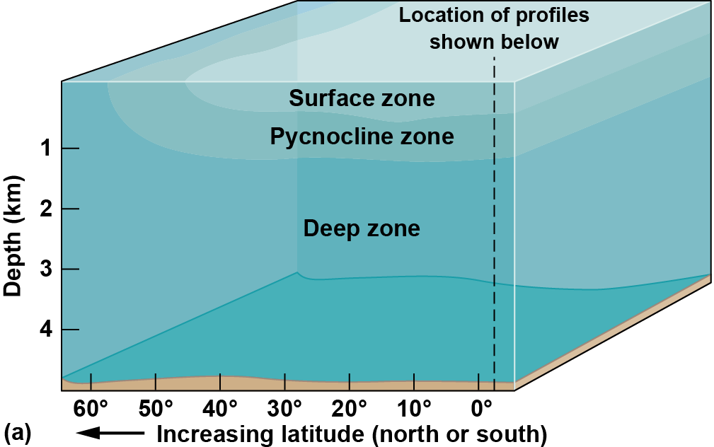
In most parts of the ocean, there is a range of depths within which density changes rapidly with depth (Fig. 8-5). Such vertical density gradients are called pycnoclines (CC1). In most parts of the open ocean, a permanent pycnocline is present with an upper boundary that is usually at a depth between 100 and 500 m. In some mid-latitude areas, another shallower seasonal pycnocline develops in summer at depths of approximately 10 to 20 m. Where a steep (large density change over a small depth increment) pycnocline occurs within the depth range of the Ekman spiral, it inhibits the downward transfer of energy and momentum. The reason is that water layers of different densities slide over each other with less friction than do water layers of nearly identical density. Water masses above and below a density interface are said to be frictionally decoupled. When a shallow pycnocline is present, the wind-driven layer is restricted to depths less than the pycnocline depth, and the Ekman spiral cannot be fully developed. Pycnoclines and the vertical structure of the ocean water column are discussed in more detail later in this chapter.

Figure 8-5. Density stratification in the oceans. (a) Throughout most of the open oceans (except in high latitudes where surface waters are cooled), a surface or mixed layer of relatively warm, nutrient-depleted, low-density water overlies a layer called the “pycnocline zone” in which density increases rapidly with depth. Below the pycnocline zone is a deep zone of cold, nutrient-rich water where density increases more slowly with depth. (b) The rapid density change with depth in the pycnocline is due primarily to changes in temperature, and the pycnocline is often called a “thermocline.” Shallow seasonal thermoclines can also develop above the main pycnocline and in coastal waters because of solar heating of the surface water. (c) In some other regions, and particularly in shallow water near major freshwater inputs, a pycnocline may develop in which the density change with depth is due to vertical variations in salinity. In this case, the pycnocline is also a “halocline.”

The Ekman spiral also cannot be fully established in shallow coastal waters because of added friction between the near-bottom current and the seafloor. Where the Ekman spiral is not fully developed because of a shallow pycnocline or seafloor, the surface current deflection is somewhat less than 45°, and Ekman transport is at an angle of less than 90° to the wind. In water only a few meters deep or less, the wind-driven water transport is not deflected from the wind direction. Instead, the current generally flows in the wind direction, but it is steered by bottom topography and flows along the depth contours.

Where Ekman transport pushes surface water toward a coast, the water surface is elevated at the coastline (Fig. 8-6a). If the Ekman transport is offshore, the sea surface is lowered at the coastline. Similarly, where Ekman transport brings surface water together from different directions, a convergence is formed at which the sea surface becomes elevated (Fig. 8-6b). In contrast, where winds transport surface water away in different directions, a divergence is formed at which the sea surface is depressed. These elevations or depressions are exaggerated in the diagrams.

Figure 8-6. Ekman transport, geostrophic currents, and Ekman circulation. (a) Where winds blow surface water shoreward, a horizontal pressure gradient develops that causes water below the surface layer to flow offshore, and water to be downwelled near the coastline. This flow is deflected by the Coriolis effect such that, if the system reaches equilibrium, the lower-layer geostrophic current flows parallel to the coast (across the pressure gradient). (b) Away from the coastline, in locations where Ekman transport of surface waters tends to create a mound of surface water at a convergence, a horizontal pressure gradient develops that causes geostrophic currents below the surface layer to flow across the pressure gradient, and water downwells at the convergence. The circulation caused by the Ekman transport, downwelling, and geostrophic flow in the lower layer is called “Ekman circulation.” Ekman circulation occurs in reverse at divergences or where winds move surface water offshore.