7.6: Interannual Climate Variations

In addition to seasonal variations, there are year-to-year and multiyear oscillations of climate that are related to ocean-atmosphere interactions. Oscillations have been identified in the tropical Pacific Ocean, the North Pacific Ocean, the Indian Ocean, the North Atlantic Ocean, and the Arctic Ocean. These may be linked with each other in ways we do not yet understand. One phase of the  oscillation in the tropical Pacific Ocean, called El Niño, is associated with climate changes affecting much of the globe and this oscillation has been extensively studied.

El Niño and the Southern Oscillation

El Niño (Spanish for “the boy”) was named because it was first observed around Christmas time off the coast of Peru. The coastal and equatorial waters off Peru are normally regions where cold water from below the ocean's surface layers is upwelled. Chapter 8 explains how winds cause this upwelling. The upwelled water contains high concentrations of nutrients that are essential to phytoplankton growth (Chap. 12). Upwelling areas therefore have high primary productivity rates, and massive schools of anchovy feed on the abundant phytoplankton that grow in the Peruvian upwelling region (Chaps. 12, 13). Until they were overfished (Chap. 16), the anchovy populations were so large that they yielded about 20% of the total world fish catch. 

Symptoms of El Niño

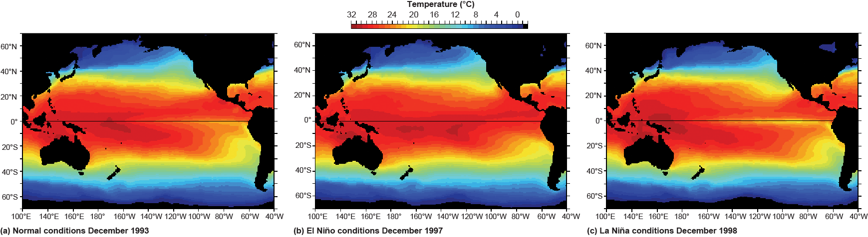
The first sign of El Niño on the Peruvian coast is a temperature change in ocean surface water. Much warmer water (5°C or more warmer) displaces the normally cold surface water (Fig. 7-18). The less dense warmer water causes stable stratification of the water column and inhibits upwelling (Chap. 8, CC1), thus reducing phytoplankton populations that were nourished by the cold upwelled water. As the phytoplankton decline, the anchovy population that feeds on them plummets, and the fishery collapses. El Niño recurs generally every 3 to 5 years and usually lasts several months until the situation reverts to neutral. El Niño events have been documented in historical records as far back as 1726.

Figure 7-18. Sea surface temperature in the Pacific Ocean, as measured by satellite-mounted sensors. (a) During non-El Niño (neutral) conditions, there is a strong band of upwelling along the equator and in the Peruvian coastal zone, which can be seen in this December 1993 image by the yellow color that indicates lower surface water temperature in these areas. (b) During a strong El Niño (December 1997), there is no upwelling along the equator, and the Peruvian coastal upwelling is greatly reduced. (c) During La Niña conditions (December 1998), the upwelling area along the equator is substantially larger, and ocean water temperature around Indonesia is higher than normal because warm surface water is driven to the west.

El Niño is not an isolated event that occurs only off the coast of Peru. In fact, it is a complex series of cyclical changes in both ocean and atmosphere that affects much of the Earth’s surface. The series of changes has been called the “El Niño/Southern Oscillation” (ENSO). The name reflects the fact that the changes in ocean and atmosphere involve a very large region of the Pacific, especially the region immediately south of the equator. The sequence of ocean-atmosphere interactions during an ENSO, now relatively well known, is described in the next section.

Between El Niños, a broad band of upwelling extends across the equatorial Pacific Ocean, and strong coastal upwelling occurs off the coast of Peru. The upwelling regions and their causes are discussed in Chapter 8. The areas of upwelling are shown by colder surface waters (Fig. 7-18a). Trade winds move warm surface water to the west, where it accumulates near Indonesia (Fig. 7-18a). An atmospheric low-pressure area is well developed in this region because of the strong evaporation from the ocean surface and the high water temperature.

The low-pressure zone normally brings plentiful rains to Indonesia and the surrounding region. In contrast, a well-developed high-pressure zone off Peru maintains low rainfall over that country, which normally has an arid climate.

Trade winds push warm water to the west, and this warm water accumulates near Indonesia, elevating sea level by as much as a few tens of centimeters in extreme cases. For reasons not yet fully understood, this situation generally begins to change from November through April. The Indonesian atmospheric low-pressure zone and the Peruvian high-pressure zone both weaken and, in some years, actually reverse. During such periods, trade winds diminish and may reverse direction for several days. Trade winds do weaken in most years and return to normal by April, but in some years the weakening trade winds are followed by an El Niño.

El Niño/Southern Oscillation Sequence

ENSO follows a relatively well-known sequence that occurs after the Indonesian low-pressure and Peruvian high-pressure systems weaken. The sequence begins as the strength of the southeast trade winds lessens in response to the weakening Peruvian high-pressure zone. The southeast trade winds are the cause of the Peruvian upwelling (Chap. 8). Therefore, the upwelling is reduced or may be stopped if the trade winds abate entirely or reverse direction.

Under neutral conditions, before an El Niño is initiated, the sea surface near Indonesia is elevated (a few tens of centimeters) in relation to the region near Peru (Fig. 7-19c). The difference is normally partially compensated for (the sea surface slope is balanced) by higher atmospheric pressure near Peru (Chap. 8, CC13). However, the atmospheric pressure difference depends on the relative strength of the Indonesian low-pressure and Peruvian high-pressure zones. Because both the high- and low-pressure zones are weakened at this stage of ENSO, the horizontal pressure change within the tropical Pacific atmosphere is too small to balance the sea surface slope and surface water flows toward the east to lower the slope.

Figure 7-19. One possible model for the development of El Niño. (a) The area of the Pacific Ocean where El Niño develops. (b) When trade winds are strong, during neutral and La Niña phases, warm surface water is pushed westward and piles up on the western boundary of the Pacific Ocean near Indonesia. The surface layer is thinned near Peru, and upwelling occurs. (c,d) Vertically exaggerated cross sections show a simplified model of the interaction of trade winds with sea-level and thermocline depth in the two extreme modes of ENSO. The cross-section in part (c) shows the effect of strong trade winds on the sea surface and surface water layer. This is the normal, or in extreme cases, the La Niña phase. (d) When the trade winds diminish, surface layer water is transported eastward toward Peru, resulting in the El Niño phase. During an El Niño, the surface layer thickens near Peru, and upwelling ceases.

In response, warm surface water from the western tropical Pacific flows eastward toward Peru (Fig. 7-19d). The flow has characteristics of an extremely long-wavelength wave that travels directly from west to east along the equator, where there is no Coriolis Effect (CC12). Therefore, the wave is free to flow across the entire ocean without deflection. This is one of the unique characteristics of ENSO. The warm surface water flows eastward across the Pacific Ocean over the cold upwelled water that is normally found in this region (Fig. 7-18b). The warmer, less dense surface water arrives near Peru and establishes a steep pycnocline in December, about 9 months after the event has started. Because steep pycnoclines are effective barriers to vertical mixing and water movements, the Peruvian coastal and tropical Pacific upwelling is further inhibited.

El Niño usually persists for about 3 months, but in extreme cases it may last 15 months or more. It ends when the reestablished trade winds again begin to drive the warm surface water of the tropical region to the west, thus restarting the upwelling process near Peru.

The oscillation set in motion by El Niño sometimes appears to “overshoot” as the system recovers. The trade winds become stronger, the water near Indonesia becomes warmer, and upwelling is stronger and water temperature lower near Peru (Fig. 7-18c). In addition, the low-pressure zone near Indonesia and the high-pressure zone near Peru become especially well developed. This situation is known as La Niña (“the girl”), in contrast to El Niño (“the boy”).

Effects of El Niño

The climatic effects of El Niño are felt far beyond the tropical Pacific. It appears that the extended area of warmer-than-usual tropical waters in the Pacific enhances the transfer of heat energy toward the poles. This change is manifested in many ways as the atmospheric convection cell system responds to the stimulus. El Niño differs in strength and other characteristics that make each El Niño’s effects somewhat different, but the same general pattern of effects is always present (Fig. 7-20). 

Figure 7-20. Strong El Niño events have worldwide effects that, in different areas, include droughts, excessive rainfall and floods, coastal erosion, tropical storms in areas where they do not normally occur, and various changes in terrestrial and marine ecosystems, some of which can be disastrous.

In the tropical Pacific, El Niño’s effects are sometimes devastating. Reduction of the warm-water pool and weakening of the atmospheric low near Indonesia brings droughts to this normally high-rainfall region. In contrast, Peru has heavy rains and coastal flooding as sea level rises. The sea level rises because the surface water layer is warmer and less dense than normal. Consequently, the surface layer is “thicker” than the normally higher-density and cold surface water layer. Offshore from Peru, the marine food web collapses from lack of nutrients normally supplied by upwelled waters. In extreme cases, the result can be massive die-offs of marine organisms, which decay, strip oxygen from the water, and produce foul-smelling sulfides (Chap. 12). The principal fishery, anchovy, is not the only biological resource affected. In severe El Niños, lack of food decimates the huge colonies of seabirds that live on islands near Peru, and causes penguins and marine mammals to undertake unusual migrations and probably suffer population losses.

Changes in atmospheric circulation caused by El Niño also alter ocean water temperatures in areas far from the tropical Pacific. In the particularly strong 1982–1983 El Niño, subtropical fishes were caught as far north as the Gulf of Alaska. This El Niño caused droughts in Australia, India, Indonesia, Central America, west-central South America, Africa, and Central Europe. Excessive rains in many cases plagued parts of Southeast Asia, California, the east coast of the U.S., and parts of South America, Britain, France, and the Arabian Peninsula (Fig. 7-20). La Niña, in contrast, typically brings flooding rains to India, Thailand, and Indonesia, and drought to Peru and northern Chile.

Modeling El Niño

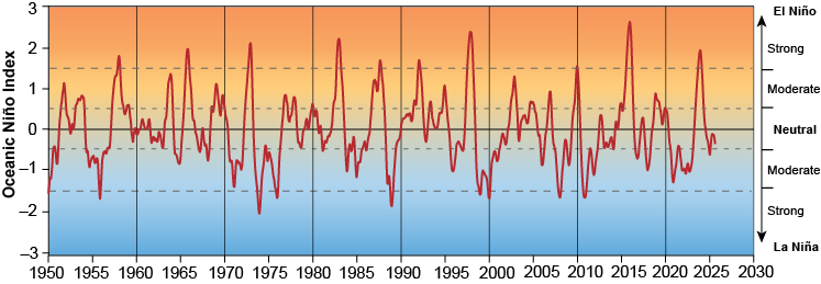
We have records of El Niños occurring regularly for centuries. La Niñas also may have occurred regularly, but they have less dramatic effects and were not recorded until scientific studies began. However, there is considerable variability from one decade to the next. In some decades, the cycle was relatively inactive; in others, it was pronounced. Since 1950, El Niño has occurred quite regularly and was followed regularly by La Niña throughout most of the period (Fig. 7-21). During the twentieth century, the strongest El Niños occurred in 1982-83 and 1997-98, and two consecutive El Niños occurred during 1991-95 without an intervening La Niña. In the first quarter of the 21st century, there were 8 El Niño episodes. The 2023-24 episode was strong, and by some definitions, the 2015-16 El Niño tied or exceeded the 1997-98 episode’s record for the strongest El Niño in recorded history. Because El Niño can have worldwide impacts on ecosystems and fisheries, and can cause widespread droughts and floods, major scientific efforts have been made to develop mathematical models (CC10) that can predict the occurrence of the phenomenon ahead of time. A number of models have been developed, each calibrated with historical data. As models have developed, they have become increasingly sophisticated, requiring increasingly detailed atmospheric and oceanic data. Gathering these data is one of the most intensive and comprehensive observational programs ever undertaken in the Earth sciences.

Figure 7-21. The NOAA Oceanic Niño Index since 1950. The index is based on the average surface water temperature in a defined region of the central tropical Pacific Ocean. El Niño (when the index rises above 0.5) and La Niña (when the index falls below –0.5) have occurred regularly about every 2–7 years.

By 1997, several models were sufficiently developed to make predictions, and all of them forecast that a modest El Niño would occur in the winter of 1997-98. The model predictions were only partly correct, as the El Niño was not a modest one. It turned out to be the most intense event on record, costing an estimated 23,000 lives and $33 billion (1998 dollars) in damage worldwide. What went wrong?

Fortunately, this El Niño was extensively observed by satellite sensors, moored instrument arrays, autonomous floats, research vessels, and aircraft. When the data were analyzed, the cause of the model failures appeared to be a burst of westerly winds in the western Pacific that occurred just as the eastward warm-water flow of the El Niño phenomenon was starting. These winds, unanticipated in the models, appear to have been timed perfectly to increase the flow of warm water across the ocean and, thus, intensify the El Niño.

Further research suggested that similar bursts of westerly winds also may have occurred just as other unusually intense El Niños had started. It has been hypothesized that these westerly winds are part of another ocean-atmosphere oscillation, called the Madden-Julian Oscillation (MJO). About every 30 days, this oscillation causes bursts of winds that are associated with an eastward-moving patch of tropical clouds. These clouds extend high into the troposphere and are easily observed from satellites. If this hypothesis is correct, the most intense El Niños may turn out to be formed only when the timing of this burst and the ENSO sequence are exactly right. The MJO cannot yet be reliably forecasted well in advance, and it may never be if the system is chaotic (CC10, CC11), which is very likely. Unfortunately, this would mean that the intensity of an El Niño could not be accurately forecast until it had already started.

El Niño Modoki

Since the early 1990s, scientists have noted a new type of El Niño that has been occurring with greater frequency and has been getting progressively stronger. In an El Niño Modoki (Japanese for “similar but different”), the maximum ocean warming is found in the central-equatorial, rather than eastern, Pacific. Such central Pacific El Niño events were observed in 1991-92, 1994-95, 2002-03, 2004-05, and 2009-10. Many of the global climate effects of an El Niño Modoki are similar to those that occur in a classic El Niño, but others are significantly different. For example, during a regular El Niño, there are generally fewer Atlantic hurricanes that make landfall in the U.S., whereas in an El Niño Modoki, there are more such hurricanes. Since detailed instrument and satellite studies of ENSO have covered only several decades, researchers are not yet sure whether El Niño Modoki is evidence of human-induced global climate change in the ENSO pattern or whether it is simply a natural long-term variability of ENSO. Some model studies have hypothesized that global warming due to human-produced greenhouse gases could shift the warming center of El Niños from the eastern to the central Pacific, further increasing the frequency of El Niño Modoki events in the future, but recent El Niños do not yet appear to show this trend.

Other Oscillations

ENSO is the best-known ocean-atmosphere oscillation, and it is believed to be the most influential in causing the interannual variations of the Earth’s climate. A number of other oscillations are known, and they too have an influence on climate, but primarily just in specific regions. The MJO, discussed in the previous section, is one such oscillation, but there are several others that have longer periods and greater effects on regional climates. These include relatively well-known oscillations in the North Atlantic and North Pacific Oceans: the North Atlantic Oscillation (NAO) and the Pacific Decadal Oscillation (PDO), respectively. More recently, oscillations have been observed in the Arctic Ocean and in the Indian Ocean. The details of what is known about these oscillations and their effects on regional climates are beyond the scope of this text. However, the following paragraphs provide a very brief overview of each.

The North Atlantic Oscillation is a periodic change in the relative strengths of the atmospheric low-pressure region centered near Iceland and the subtropical high-pressure zone near the Azores. This pressure difference drives the wintertime winds and storms that cross from west to east across the North Atlantic. When the gradient between the two zones weakens, more powerful storms create harsher winters in Europe. The shift can affect marine and terrestrial ecology, food production, energy consumption, and other economic factors in the regions surrounding the North Atlantic. The periodicity of NAO is highly variable, but it ranges from several years to a decade or more. The Arctic Oscillation is closely coupled with the NAO. The Arctic high-pressure region tends to be weak when the Icelandic low is strong. The strength of the Arctic high affects climate around the Arctic Ocean, as well as the direction and intensity of ice drift.

Two modes characterize the Pacific Decadal Oscillation. In one mode, the sea surface temperatures in the northwestern Pacific, extending from Japan to the Gulf of Alaska, are relatively warm, and the sea surface temperatures in the region from Canada to California and Hawaii are relatively cool. In the other mode, these relative temperatures are reversed. In the first mode, the jet stream flows high across the Pacific and dips south over the Pacific coast of North America. Pacific storms follow the jet stream onto the continent over Washington, Oregon, or British Columbia, and California is cool and dry. Moist, relatively warm air is transported across the northern half of the United States, resulting in relatively mild, but often wet, winters in this region and in states influenced by warm, moist air masses from the Gulf of Mexico. In the second mode, the jet stream and Pacific storm tracks parallel the Pacific coast into Canada and Alaska. Parts of Alaska and much of California experience a mild winter. However, the jet stream's location allows cold, dry Arctic air to flow over the central United States, pushing the Gulf of Mexico air mass south, and a generally cold winter occurs in the eastern United States. We discuss some of the effects of the PDO in more detail in the next section.

In the Indian Ocean, there is no strong oscillation comparable to ENSO in the Pacific. However, there is evidence of a weaker oscillation that is similar. Although the Indian Ocean oscillation, known as the Indian Ocean Dipole (IOD), is much weaker than ENSO, it exhibits similar warm, neutral, and cold phases. The warm phase is characterized by warmer water on the western side of the ocean and cooler water on the eastern side, while the cold phase has warmer water in the eastern Indian Ocean and cooler water in the west. Modeling has shown that the intense drought of 1998–2002 over a swath of mid latitudes spanning the United States, the Mediterranean, southern Europe, and Southwest and Central Asia was possibly caused by a combination of the strong El Niño of 1997-98, and the cool phase of the IOD oscillation in the Indian Ocean.

Climate Chaos?

The decade following the 1976-77 winter was extremely unusual in the U.S. and elsewhere. For example, in the following eight years, five severe freezes damaged Florida orange groves. Such freezes had occurred, on average, only once every 10 years over the previous 75 years. In addition, waves 6 m or higher tore into the southern California coastline 10 times in the 4 years from 1980 to 1984. Such waves had occurred there only 8 times in the preceding 80 years.

Were all these “unusual” events the result of a sudden shift in climate or just due to normal year-to-year variations of the Earth’s climate? Because any one such change could be just a year-to-year variation, researchers examined the records of 40 different environmental variables that reflect climatic conditions around the Pacific region. The variables include wind speeds in the subtropical North Pacific Ocean, the concentration of chlorophyll in the central North Pacific Ocean, the salmon catch in Alaska, the sea surface temperature in the northeastern Pacific, and the number of Canada goose nests on the Columbia River. The 40 variables were combined to derive a single statistical index of climate for each year from 1968 to 1984.

The index showed a distinct and abrupt step-like change in value between 1976 and 1977, which is truly remarkable because such a clear signal of changed conditions is seldom, if ever, found even in any single environmental variable. Usually the many complex natural variations would obscure such a pattern. Was this change real? Did it indicate a chaotic “phase shift” between two relatively stable sets of environmental conditions? This study was perhaps the first evidence that chaotic shifts do indeed occur. It later became known that this shift was associated with the Pacific Decadal Oscillation (PDO), named in 1997. In 2000, this study was repeated, but this time using as many as 100 variables: 31 time series of atmospheric or oceanic physical variables, such as indices of the sea surface temperature; and 69 biological time series, such as catch rates of salmon. The analysis was performed for the period 1965–1995, but because data were not available for all indices for each year, the analysis was done in two blocks—1965–1985 and 1985–1995—using a slightly different suite of indices for each. The results were as startling as those of the early studies. Distinct phase shifts were identified between 1976 and 1977, and between 1988 and 1989 (Fig. 7-22). These dates correspond with reversals of the PDO. Further evidence that these phase shifts may involve elements of chaos comes from the observation that some of the individual biological indices that changed in 1997 did not simply reverse in 1989. Indeed, some made step increases in both years, and some made step decreases in both years. These observations indicate that some species did not return to their former numbers in the ecosystem. This indicates that atmospheric oscillation driven shifts may be an agent of long-term change in the success of individual species within ocean and, perhaps, terrestrial ecosystems.

Figure 7-22. Variations in a composite index of environmental variables related to climate in the North Pacific Ocean. Time series were examined for 100 variables—31 climatic and 69 biological—although data were not available for all variables throughout the analysis period. (a) A regime shift occurred in the winter of 1976–1977, as shown by the step change in this function, which includes time series for 91 variables. (b) A regime shift also occurred in 1989, as shown by the step decrease in an index that includes time series for 94 variables. However, this second shift did not restore the system to its pre-1977 state.

If changes in the Earth’s ocean-atmosphere climate system and associated ecological effects are chaotic, what does this mean? Chaotic systems often remain stable, varying within a well-defined range of behaviors, until the entire system suddenly shifts to a new stable state and varies within a different range of behaviors (CC11). Thus, it may mean that ecosystems are constantly changing in unpredictable ways. It may also mean that, even if no dramatic climate changes have yet occurred in response to human releases of greenhouse gases, there is no guarantee that any future changes will be small or slow. Drastic, sudden climate changes could be triggered if greenhouse gas concentrations in the atmosphere continue to increase, or they may already be inevitable. Decades of research on the Earth’s ocean-atmosphere climate system are needed before we can have confidence in any forecasts of future climate in a world in which we have caused an unprecedented, rapid increase in the concentration of greenhouse gases in the atmosphere. Furthermore, such forecasts may never be more reliable than the local weather forecast.