3.3: Bathymetry

People have long needed to map seafloor topography to navigate safely past obstructions such as submerged rocks and reefs. They have also long been curious about the depth of water over the seafloor. 

Soundings

For centuries, the only way to explore any seafloor deeper than the few tens of meters that could be reached by pearl divers or in crude diving bells was by lowering a line into the water with a weight attached. The length of line payed out (on a ship, letting out line is referred to as “paying out”) before the weight hit the bottom indicated the water depth—a measurement called a sounding. This method led to the unit of depth called the “fathom,” which was used almost exclusively for nautical charts until it was supplanted in recent decades by the meter. The fathom was originally 5.5 ft., or the length of line between the outstretched arms of the man hauling the sounding line back aboard the ship. Originally, all depths were measured as a count of the number of such lengths of line that were hauled back aboard after the sounding weight hit the bottom. Later the fathom was changed to exactly 6 ft., and sounding lines, particularly those used for deeper soundings, had knots or ribbons tied at measured intervals to improve the sounding accuracy.

A modification of sounding with line and weight was used to collect samples of bottom sediment. The bottom of the weight, usually lead, was hollowed out and fitted with a lump of tallow. When the tallow hit the bottom, a small amount of bottom sediment adhered to it, unless the weight hit a rocky bottom. Early nautical charts included a description of the type of seafloor based on such samples. Seafloor composition was categorized as sand, silt, or mud, with the mud color sometimes noted. Many modern nautical charts, particularly those of shallow coastal waters, still include that information.

Sounding technology saw a major technological advance during the 1885 voyage of the USS Tuscarora to study possible routes for a telephone cable between America and Japan. On the ship’s voyage, the sounding line was replaced by a single strand of piano wire with a weight attached at its end. The wire was deployed from a drum and hauled back by a winch. Because hauling with a winch was much faster than hand-hauling, the Tuscarora could make several deep soundings each day. Despite this improvement, fewer than 6000 soundings had been made in depths greater than 1000 fathoms (1800 m) by 1910. Hence, fewer than 6000 depth measurements had been made in an area that covers approximately 40% of the Earth’s surface—an area nearly 30 times larger than the combined surface area of the 48 contiguous U.S. states. Knowledge of the topography of the deep-ocean floors was only rudimentary, even as late as the beginning of World War I in 1914. For comparison, consider a map of the mountains, plains, and river valleys of the U.S. if the country were covered in clouds and had been studied solely by lowering a wire through the clouds to the ground at only 200 locations.

Sounding Errors and Problems

Taking soundings using a line or wire is a tedious process that poses additional problems, many of which must still be overcome when wires are being used to lower instrument packages. For example, determining when the weight on the wire has reached the bottom is difficult in deep water. Several kilometers of line or wire is sufficiently heavy to continue to pull more wire from the drum, even when the weight at the end has hit the bottom. Watching for a reduction in how fast the wire pays out or for a slackening of the tension in the wire, each of which occurs when weight is reduced by bottom impact, can sometimes help to overcome this problem. However, these techniques are very difficult, especially in bad weather, even using electronic wire-tension measurement systems. As the ship rolls, the head of the crane or the A-frame over which the wire is payed out moves up and down in relation to the sea surface. When a considerable length of wire has been payed out, its weight and drag in the water prevent it from moving up and down with the ship’s roll. As a result, it stretches and contracts, and the wire tension fluctuates. Therefore, wires must be several times stronger than would be necessary to carry only their own weight and the weight of any instruments attached to them.

When wires are used to lower instruments, currents and wind blowing against the research vessel can also cause problems. Because the ship is slowly blown along the sea surface by the wind, it tends to move sideways from the weight or instrument package on the wire that is far below. The drag of the wire and its weight tend to prevent the wire from following the ship’s sideways motion. Therefore, the wire does not drop vertically to the bottom (Fig. 3-2). If subsurface currents flow in a different direction from the research vessel’s wind drift, or from that of currents at other depths, the wire’s vertical path through the water can have a complex S shape or other curve (Fig. 3-2). Because a wire never falls through a deep water column vertically, more wire than the actual water depth beneath the research vessel must be let out if the end of the wire is to reach the seafloor. Therefore, all line and wire soundings in deep water were incorrect. The actual depth was always less than the measured depth.

Figure 3-2. Winds and currents can deform the vertical path of a sounding weight or instrument package on the end of a wire as it falls to the seafloor. Currents in the surface layer or winds that blow the vessel across the ocean surface can move the vessel away from the vertical path of the weight. Therefore, a length of wire longer than the water’s depth must be payed out for the instruments to reach the seafloor. Currents in lower layers can further complicate the path of the wire, particularly in very deep water where several kilometers of wire must be payed out for the instrument package to reach the seafloor.

A more practical problem associated with lowering instruments or wires over the side of a research vessel is that the wind or currents can blow the vessel over the top of the wire or bend the wire under the vessel. The wire can end up stretched tight against the curve of the ship’s hull as it passes underneath. Continuing to lower or raise the wire in this situation could damage the ship’s hull or break the wire. Therefore, most oceanographic research vessels are specifically designed to be capable of turning slowly around the wire without moving forward. This ability is usually provided by a bow thruster propeller located in a tunnel near the bow of the ship. The propeller is set at a right angle to the ship’s normal direction of travel and can be used to push the bow of the ship to one side or the other.

Echo Sounders

In response to the sinking of the Titanic in 1912, Reginald Fessender, a former assistant to Thomas Alva Edison, invented a device that could detect an iceberg almost 5 km away by sending a sound signal through the water and detecting the return echo. That sound navigation and ranging equipment, which became known as sonar, was quickly developed into a device for hunting submarines during World War I. After the invention of sonar, it was a simple matter to orient the sound source to point vertically downward (Fig. 3-3) and to detect the echo from the seafloor. The speed of sound in seawater is known, as are the relatively small changes in this speed with salinity and temperature. Hence, if the distribution of salinity and temperature with depth is known from other measurements, the depth of the water below a ship can be determined by measurement of the time taken for the sound to travel to the seafloor and back. The first truly successful echo sounder depth recordings were made in the North Sea in 1920 by the German scientist Alexander Behm. Subsequently, knowledge of bottom topography developed rapidly as echo sounding equipment was improved and installed in more vessels.

Figure 3-3. Echo sounders measure the depth of water beneath a vessel by measuring how much time a sound pulse takes to travel from the vessel to the seafloor and back. Because sound travels in seawater at about 1500 m•s–1, a sound pulse takes 2 s to return to the research vessel when the water depth is 1500 m. The sound pulses spread out over a narrow angle as they travel downward from the vessel. Thus, in deep water, they are reflected off a large area of seafloor.

The great advantage of echo sounders was that they could obtain essentially continuous records of the water depth below a moving ship. By the mid-twentieth century, every research vessel was equipped with an extremely precise echo sounder called a “precision depth recorder” (PDR). Standard operating procedures on most research vessels required that the PDR be operated continuously, and that depths and precise ship positions be recorded while the vessel was under way. PDR depth measurements, although much more accurate than soundings, also have limitations. Because the PDR records only the depth of water directly under the ship’s track, depths between two ship tracks still must be inferred by interpolation. Unless depth recordings from many ship tracks cover a given area of ocean floor, major features such as undersea hills and mountains may still be overlooked. In addition, the PDR measures only the depth of the closest echo from under the vessel (Fig. 3-3). Even PDRs with very narrow beam widths receive echoes from a relatively large area of ocean floor. Hence, a nearby hill can cause the depth to be recorded as shallower than it really is, and narrow valleys and depressions can be missed completely (Fig. 3-3).

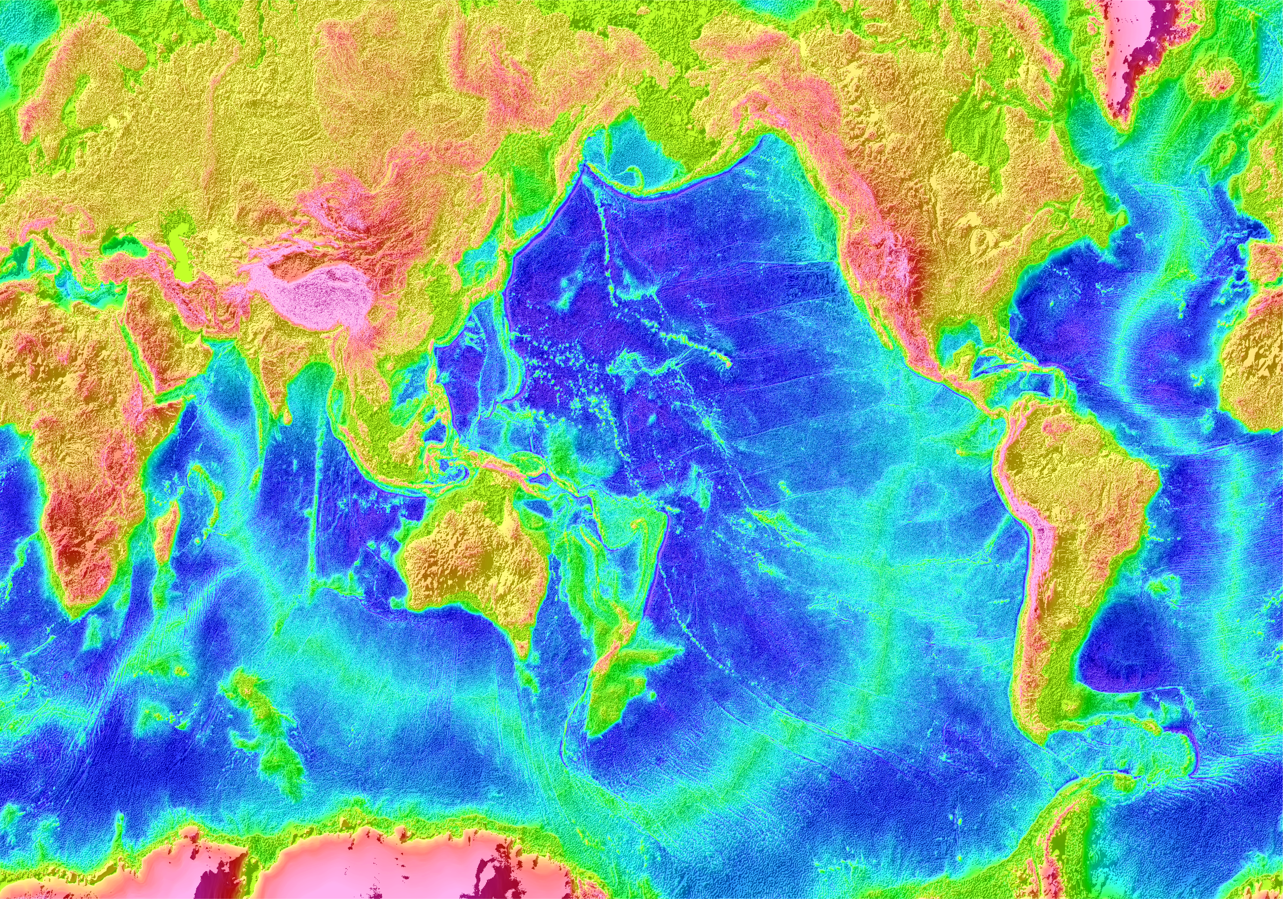
The depth information generated by research vessels after World War II had to be plotted by hand, which proved to be a daunting task. Of course, depths are now recorded electronically and processed by computers, but computers did not become practical for use at sea until the 1970s. The first truly comprehensive map of the ocean floor was completed by Bruce Heezen and Marie Tharp in 1959. Compiling it was an enormous and tedious undertaking that involved matching depth and position (navigation) data from thousands of hours of PDR recordings made by many vessels without the aid of computers. Navigation errors were corrected by comparison of the depths of each ship, recorded where ship track lines crossed. Depth data were then entered painstakingly on a blank map and carefully contoured, and then a three-dimensional representation was drawn exactingly by hand. The map generated by this massive project was truly revolutionary.

To understand this, look at a typical atlas map that shows all the oceans as a featureless uniform blue expanse, then look at Figure 3-4. This revelation of previously unseen seafloor topography that rivals the greatest mountain chains and other features of the continents was, for oceanographers and others, like being introduced to an entirely new planet. Heezen and Tharp, and the many other people who spent years gathering data or otherwise helping to create the map, made a contribution to human knowledge that today remains startling, profound, and beautiful.

Figure 3-4. Mercator projection map of the seafloor and land surface elevation. Seafloor elevation data were obtained from ship generated precision depth recorder data and satellite measurements of sea surface height data. (Data were obtained from many sources.) The highest resolution sea surface height data used in this map was from satellites, permitting only features greater than about 20–25 km across to be shown in this map. Click for a larger version of the map.

Since 1959, PDR surveys of the oceans have continued on almost all research vessels during their entire time at sea. Nevertheless, most of the ocean floor is still very poorly mapped by this technique. In fact, vast areas of the deep oceans have been mapped by PDRs at a level of detail equivalent to mapping the U.S. only by measuring elevations along the interstate highways. Look at a road atlas and think about what topography we would have missed if we had mapped the U.S. from topographic data taken only along this highway system.

Wide-Area Echo Sounders

In the 1960s, echo sounding was revolutionized by the simultaneous development in the U.S. and England of somewhat different approaches to determining the seafloor topography within a wide swath under, and to either side of, a vessel track. In the American system, called “multibeam sonar” or “swath,” up to 200 or more narrow sound beams are broadcast in a fan pattern beneath the ship (Fig. 3-5a), and the depth (corrected for the angle) is recorded for each beam. In the British system, called “sidescan sonar,” two wider sound beams are broadcast at an angle, one to each side and downward from a streamlined instrument enclosure called a “fish” towed underwater behind the vessel (Fig. 3-5b). In this system, echoes from different broadcast angles within each beam return to the fish at different times, depending on the angle and therefore the distance from the fish. Within the prolonged returning sequence of echoes from each outgoing pulse, the intensity of the echo received varies according to distance and the bottom topography. Strong portions of the returning echo sequence indicate that the bottom is sloped up toward the fish. Weak echoes indicate an area sloped down away from the fish. These represent the front and back sides of the hill, respectively.

Figure 3-5. Modern seafloor topography measurements have been continuously improving and are now made with two different systems. (a) Sidescan sonar uses a broad sound beam sent from a towed fish. (b) Multibeam sonar systems use up to 1000 or more separate narrow beams spread out under the ship or towed fish. Both systems require computer processing of return echo data produce much more detailed seafloor maps than were previously possible. (c) The colored area of this map shows the detailed topography revealed by a multibeam sonar survey of Quick’s Hole, Massachusetts in 2004. The surrounding white nautical chart shows the much less detailed maps that were available before sidescan or multibeam sonar were developed. (d) This multibeam image of a deep-water ridge north of Sulawesi Island, Indonesia from a scan taken in 2010 shows the improvement in sonar systems.

The two wide-area echo sounding systems have somewhat different uses because each is better suited to mapping certain types of bottom terrain in certain depths of water depths. Each system requires powerful and sophisticated computer technology to process the signals received. Both methods provide dramatically improved maps and reveal previously unknown canyons, valleys, hills, and other features of the seafloor (Fig. 3-5c). Detailed charts of coastal waters developed with the new echo sounding systems are now being produced as each area is surveyed. 

In the early part of this century, side scan sonar evolved into a newer system, synthetic aperture sonar (SAS). The main difference between side scan sonar and SAS is that SAS uses sophisticated signal processing to coherently recombine the overlapping areas of the pings to create ultra-high resolution images (Figure 3-6c). The return echo data are then mathematically combined for up to several successive pings. This requires far more computing power than even side scan sonar requires but results in a far more detailed view of the seafloor (Figure 3-6). SAS provides greater resolution than side-scan over a comparable area, more information about the sediment type, and details of small objects such as fish holes and burrows. While the resolution of side scan tends to degrade with distance between seafloor and the towed fish, SAS systems have a consistent resolution throughout the full operational range. The resolution of these systems can be degraded by random motions such as those that occur during bad weather when a ship and its towed array are affected by wave and wind action. SAS is now used extensively in marine archaeological surveys, and military applications such as mine detection.

Figure 3-6. (a) Multibeam and sidescan sonar both rely on successive pings and return echos that are timed so there is minimal overlap, and the echo from each ping is computer processed separately. (b) Synthetic aperture sonar pings more often, causing the echo return areas from two or more successive pings to overlap. More complex computations then analyze the data by combining the echo returns from two or more pings. The following parts of this figure show the differences in resolution between the sonar types taken at the same distance from the seafloor (c) Multibeam and sidescan sonar can resolve objects about 1 m across. (d) Synthetic aperture sonar, when processed to extract bathymetric data, can resolve objects several times smaller, and (d) when processed as an image, can resolve objects just a few centimeters across. [Images courtesy of Kraken Robotics]

Multibeam, sidescan, and synthetic aperture sonar are now generally mounted in AUVs as each type of sonar is sensitive to the motions of a ship or towed fish. Also AUV’s, which are discussed more later in the chapter, can fly at depth, closer to the seabed being surveyed, and they can survey an area without the need for constant attention from a surface vessel. Such systems can now operate at depths of up to 6,000 m but are expensive to build and operate. Although these systems are beginning to expand the area in which the ocean floor is surveyed in detail, it will still take decades or longer before the majority of the seafloor is surveyed at the level of detail possible with sidescan, multibeam, or synthetic aperture sonar. 

Ocean Topography from Satellites

Unlike research vessels and autonomous floats, satellites have been able to survey the world’s oceans with unprecedented comprehensiveness in just a few days, albeit at lower resolution than sonar can achieve.

The Seasat satellite launched in 1978 made the first satellite-based maps of the ocean surface, from which the topography of the seafloor can be deduced. The sea surface topography was measured by a radar altimeter carried on board the satellite. The height of the sea surface can be used to map the seafloor topography because it is affected by the depth of the ocean below it. Rock is denser than water, so rocks have a slightly higher gravitational attraction than water. Therefore, the sea surface is slightly higher over an undersea mountain than it is over a deeper area (the mountain “pulls” water toward it from the sides to create “mounds”). There are now several satellites in orbit that provide satellite altimetry data and made it possible to map the entire world’s ocean floor. This data has led to the discovery of hundreds of previously unknown seamounts, fracture zones, and other topographic features in areas where depth recordings had not been made by ships. By 2023, high resolution radar satellites had identified more than 43,000 seamounts of which only about 16,000 have been mapped by sonar.

Data from satellites and from shipboard PDR surveys have all been combined to provide a detailed view of the ocean floor (Fig. 3-4). However, the resolution of these maps is still such that features as large as several kilometers across may be missed. Limitations inherent to satellite bathymetry make it unlikely that substantially better resolution will ever be obtained except where detailed wide-area sonar surveys are made.

In contrast to ocean floor mapping, scientists completed the mapping of other planets and their moons quickly and easily using radar, cameras, and modern computers aboard planetary probes such as the Mariner, Voyager, and Mars Global Surveyor spacecraft. In addition, the resolution and comprehensiveness of our maps of Mars, Venus, and the Earth’s moon are much better than our seafloor maps. This comparison illustrates the difficulty of studying the oceans.