6.4: Lab Exercise (Part A, B, and C)
- Page ID
- 5560
\( \newcommand{\vecs}[1]{\overset { \scriptstyle \rightharpoonup} {\mathbf{#1}} } \)
\( \newcommand{\vecd}[1]{\overset{-\!-\!\rightharpoonup}{\vphantom{a}\smash {#1}}} \)
\( \newcommand{\id}{\mathrm{id}}\) \( \newcommand{\Span}{\mathrm{span}}\)
( \newcommand{\kernel}{\mathrm{null}\,}\) \( \newcommand{\range}{\mathrm{range}\,}\)
\( \newcommand{\RealPart}{\mathrm{Re}}\) \( \newcommand{\ImaginaryPart}{\mathrm{Im}}\)
\( \newcommand{\Argument}{\mathrm{Arg}}\) \( \newcommand{\norm}[1]{\| #1 \|}\)
\( \newcommand{\inner}[2]{\langle #1, #2 \rangle}\)
\( \newcommand{\Span}{\mathrm{span}}\)
\( \newcommand{\id}{\mathrm{id}}\)
\( \newcommand{\Span}{\mathrm{span}}\)
\( \newcommand{\kernel}{\mathrm{null}\,}\)
\( \newcommand{\range}{\mathrm{range}\,}\)
\( \newcommand{\RealPart}{\mathrm{Re}}\)
\( \newcommand{\ImaginaryPart}{\mathrm{Im}}\)
\( \newcommand{\Argument}{\mathrm{Arg}}\)
\( \newcommand{\norm}[1]{\| #1 \|}\)
\( \newcommand{\inner}[2]{\langle #1, #2 \rangle}\)
\( \newcommand{\Span}{\mathrm{span}}\) \( \newcommand{\AA}{\unicode[.8,0]{x212B}}\)
\( \newcommand{\vectorA}[1]{\vec{#1}} % arrow\)
\( \newcommand{\vectorAt}[1]{\vec{\text{#1}}} % arrow\)
\( \newcommand{\vectorB}[1]{\overset { \scriptstyle \rightharpoonup} {\mathbf{#1}} } \)
\( \newcommand{\vectorC}[1]{\textbf{#1}} \)
\( \newcommand{\vectorD}[1]{\overrightarrow{#1}} \)
\( \newcommand{\vectorDt}[1]{\overrightarrow{\text{#1}}} \)
\( \newcommand{\vectE}[1]{\overset{-\!-\!\rightharpoonup}{\vphantom{a}\smash{\mathbf {#1}}}} \)
\( \newcommand{\vecs}[1]{\overset { \scriptstyle \rightharpoonup} {\mathbf{#1}} } \)
\( \newcommand{\vecd}[1]{\overset{-\!-\!\rightharpoonup}{\vphantom{a}\smash {#1}}} \)
\(\newcommand{\avec}{\mathbf a}\) \(\newcommand{\bvec}{\mathbf b}\) \(\newcommand{\cvec}{\mathbf c}\) \(\newcommand{\dvec}{\mathbf d}\) \(\newcommand{\dtil}{\widetilde{\mathbf d}}\) \(\newcommand{\evec}{\mathbf e}\) \(\newcommand{\fvec}{\mathbf f}\) \(\newcommand{\nvec}{\mathbf n}\) \(\newcommand{\pvec}{\mathbf p}\) \(\newcommand{\qvec}{\mathbf q}\) \(\newcommand{\svec}{\mathbf s}\) \(\newcommand{\tvec}{\mathbf t}\) \(\newcommand{\uvec}{\mathbf u}\) \(\newcommand{\vvec}{\mathbf v}\) \(\newcommand{\wvec}{\mathbf w}\) \(\newcommand{\xvec}{\mathbf x}\) \(\newcommand{\yvec}{\mathbf y}\) \(\newcommand{\zvec}{\mathbf z}\) \(\newcommand{\rvec}{\mathbf r}\) \(\newcommand{\mvec}{\mathbf m}\) \(\newcommand{\zerovec}{\mathbf 0}\) \(\newcommand{\onevec}{\mathbf 1}\) \(\newcommand{\real}{\mathbb R}\) \(\newcommand{\twovec}[2]{\left[\begin{array}{r}#1 \\ #2 \end{array}\right]}\) \(\newcommand{\ctwovec}[2]{\left[\begin{array}{c}#1 \\ #2 \end{array}\right]}\) \(\newcommand{\threevec}[3]{\left[\begin{array}{r}#1 \\ #2 \\ #3 \end{array}\right]}\) \(\newcommand{\cthreevec}[3]{\left[\begin{array}{c}#1 \\ #2 \\ #3 \end{array}\right]}\) \(\newcommand{\fourvec}[4]{\left[\begin{array}{r}#1 \\ #2 \\ #3 \\ #4 \end{array}\right]}\) \(\newcommand{\cfourvec}[4]{\left[\begin{array}{c}#1 \\ #2 \\ #3 \\ #4 \end{array}\right]}\) \(\newcommand{\fivevec}[5]{\left[\begin{array}{r}#1 \\ #2 \\ #3 \\ #4 \\ #5 \\ \end{array}\right]}\) \(\newcommand{\cfivevec}[5]{\left[\begin{array}{c}#1 \\ #2 \\ #3 \\ #4 \\ #5 \\ \end{array}\right]}\) \(\newcommand{\mattwo}[4]{\left[\begin{array}{rr}#1 \amp #2 \\ #3 \amp #4 \\ \end{array}\right]}\) \(\newcommand{\laspan}[1]{\text{Span}\{#1\}}\) \(\newcommand{\bcal}{\cal B}\) \(\newcommand{\ccal}{\cal C}\) \(\newcommand{\scal}{\cal S}\) \(\newcommand{\wcal}{\cal W}\) \(\newcommand{\ecal}{\cal E}\) \(\newcommand{\coords}[2]{\left\{#1\right\}_{#2}}\) \(\newcommand{\gray}[1]{\color{gray}{#1}}\) \(\newcommand{\lgray}[1]{\color{lightgray}{#1}}\) \(\newcommand{\rank}{\operatorname{rank}}\) \(\newcommand{\row}{\text{Row}}\) \(\newcommand{\col}{\text{Col}}\) \(\renewcommand{\row}{\text{Row}}\) \(\newcommand{\nul}{\text{Nul}}\) \(\newcommand{\var}{\text{Var}}\) \(\newcommand{\corr}{\text{corr}}\) \(\newcommand{\len}[1]{\left|#1\right|}\) \(\newcommand{\bbar}{\overline{\bvec}}\) \(\newcommand{\bhat}{\widehat{\bvec}}\) \(\newcommand{\bperp}{\bvec^\perp}\) \(\newcommand{\xhat}{\widehat{\xvec}}\) \(\newcommand{\vhat}{\widehat{\vvec}}\) \(\newcommand{\uhat}{\widehat{\uvec}}\) \(\newcommand{\what}{\widehat{\wvec}}\) \(\newcommand{\Sighat}{\widehat{\Sigma}}\) \(\newcommand{\lt}{<}\) \(\newcommand{\gt}{>}\) \(\newcommand{\amp}{&}\) \(\definecolor{fillinmathshade}{gray}{0.9}\)Overview
As with Chapter 4, you will be expected to input your answers to this lab in several ways. There will be a couple of multiple-choice questions, but for the majority of the lab you will write your answers in the provided text box. This allows you to show your work in the questions requiring calculations as well as allowing you to answer open-ended questions thoroughly with multiple sentences. You will be expected to use correct grammar and complete sentences in your answers.
Materials
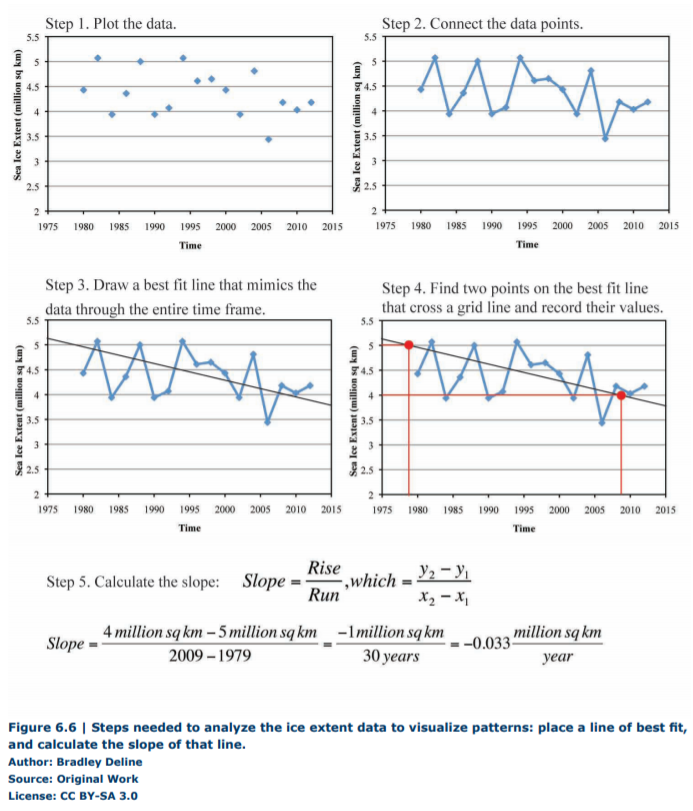
All of the data provided in the lab comes from the National Snow and Ice Data Center (NSIDC), housed at the University of Colorado. The data presented in this lab can be freely downloaded from them at nsidc.org. The original discussion was focused on a widely circulated though unattributed article entitled “Antarctic Sea Ice for March 2010 Significantly Greater Than 1980” published in April 2010 (climatechangehoax.com). For the dataset presented in this article as well as the following datasets, do the following before answering each set of questions: graph the data, connect the data points to better see the pattern through time, estimate the best fit line, and calculate the slope of the best fit line. Make sure to think about the data before you estimate the line of best fit so that your line falls within the data and is consistent with the trend in the data. An example of this process is shown in Figure 6.6.
Part A – Original Data
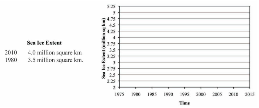
First, we want to take a closer look at the data presented in the original article (“Antarctic Sea Ice for March 2010 Significantly Greater Than 1980”) and interpret the data. Feel free to read the article, but it isn’t needed to complete the assignment or understand the patterns it is presenting. The data, which is included to the left of the graph below, is the extent of Antarctic sea ice in millions of square kilometers as measured in March of 1980 and 2010. This data is accurate and is consistent with data that can be downloaded from NSIDC. To do this, follow the instructions in Figure 6.6. In this case, steps two and three are the same and you can easily calculate slope using the original data.
1. Based exclusively on the data provided and your graph, what conclusion would you make regarding climate change?
a. Sea ice is expanding, which indicates an increase in temperature.
b. Sea ice is expanding, which indicates a decrease in temperature.
c. Sea ice is contracting, which indicates an increase in temperature.
d. Sea ice is contracting, which indicates a decrease in temperature.
2. What is slope of the line of best fit for this data?
a. 0.008 million square kilometers per year
b. 0.05 million square kilometers per year
c. -0.05 million square kilometers per year
d. 0.017 million square kilometers per year
e. -0.17 million square kilometer per year
f. 0.033 million square kilometer per year
3. Even though the above data is accurate, give and explain two reasons why this dataset might lead you to an incorrect conclusion regarding global climate change.
Part B – South Pole Sea Ice Extent
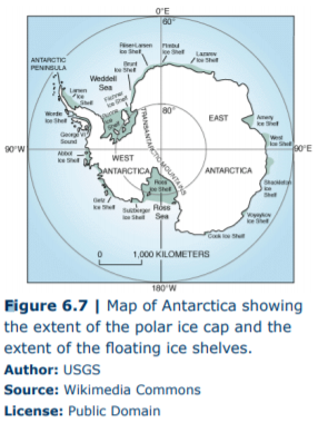
Below is an expanded dataset showing Antarctic sea ice (Figure 6.7) extent measured during March 1980 through 2012 again downloaded from NSIDC. Only the even-numbered years are presented, but the addition of odd years does not alter the trend in the data. Following the instructions in Figure 6.6, graph the data, draw a line of best fit, and calculate the slope of the line.
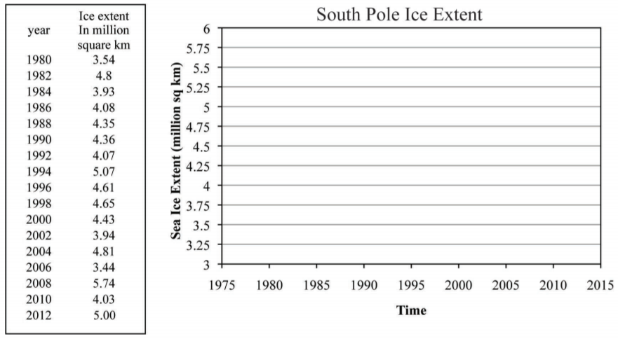
4. What is the slope of the line of best fit you estimated for this data set? Make sure to show your work.
5. What conclusion about climate change could you make from this dataset? How does your result for the extended dataset compare to the results from the data presented in the article (Part A)?
Part C – North Pole Sea Ice Extent
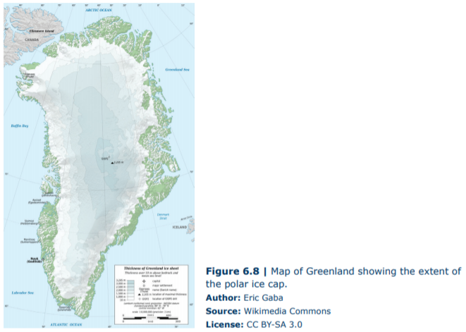
Next, we will examine the ice extent patterns of the northern Arctic polar ice sheet that is located around Greenland (Figure 6.8). The ice extent data is from March 1980 through 2012, for even-numbered years, again downloaded from NSIDC. Following the instructions in Figure 6.6, graph the data, draw a line of best fit, and calculate the slope of the line.
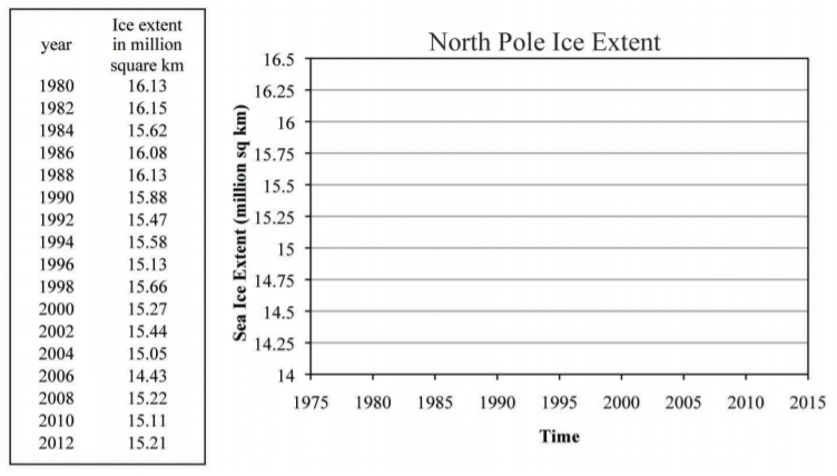
6. What is the slope of the line of best fit you estimated for this data set? Make sure to show your work.
7. What conclusion on climate change could you make from this dataset? How does your result for the North Pole compared to that of the South Pole (Part B)?


