
5.6: Lab Exercise (Part B)
- Page ID
- 5508

\( \newcommand{\vecs}[1]{\overset { \scriptstyle \rightharpoonup} {\mathbf{#1}} } \)
\( \newcommand{\vecd}[1]{\overset{-\!-\!\rightharpoonup}{\vphantom{a}\smash {#1}}} \)
\( \newcommand{\id}{\mathrm{id}}\) \( \newcommand{\Span}{\mathrm{span}}\)
( \newcommand{\kernel}{\mathrm{null}\,}\) \( \newcommand{\range}{\mathrm{range}\,}\)
\( \newcommand{\RealPart}{\mathrm{Re}}\) \( \newcommand{\ImaginaryPart}{\mathrm{Im}}\)
\( \newcommand{\Argument}{\mathrm{Arg}}\) \( \newcommand{\norm}[1]{\| #1 \|}\)
\( \newcommand{\inner}[2]{\langle #1, #2 \rangle}\)
\( \newcommand{\Span}{\mathrm{span}}\)
\( \newcommand{\id}{\mathrm{id}}\)
\( \newcommand{\Span}{\mathrm{span}}\)
\( \newcommand{\kernel}{\mathrm{null}\,}\)
\( \newcommand{\range}{\mathrm{range}\,}\)
\( \newcommand{\RealPart}{\mathrm{Re}}\)
\( \newcommand{\ImaginaryPart}{\mathrm{Im}}\)
\( \newcommand{\Argument}{\mathrm{Arg}}\)
\( \newcommand{\norm}[1]{\| #1 \|}\)
\( \newcommand{\inner}[2]{\langle #1, #2 \rangle}\)
\( \newcommand{\Span}{\mathrm{span}}\) \( \newcommand{\AA}{\unicode[.8,0]{x212B}}\)
\( \newcommand{\vectorA}[1]{\vec{#1}} % arrow\)
\( \newcommand{\vectorAt}[1]{\vec{\text{#1}}} % arrow\)
\( \newcommand{\vectorB}[1]{\overset { \scriptstyle \rightharpoonup} {\mathbf{#1}} } \)
\( \newcommand{\vectorC}[1]{\textbf{#1}} \)
\( \newcommand{\vectorD}[1]{\overrightarrow{#1}} \)
\( \newcommand{\vectorDt}[1]{\overrightarrow{\text{#1}}} \)
\( \newcommand{\vectE}[1]{\overset{-\!-\!\rightharpoonup}{\vphantom{a}\smash{\mathbf {#1}}}} \)
\( \newcommand{\vecs}[1]{\overset { \scriptstyle \rightharpoonup} {\mathbf{#1}} } \)
\( \newcommand{\vecd}[1]{\overset{-\!-\!\rightharpoonup}{\vphantom{a}\smash {#1}}} \)
\(\newcommand{\avec}{\mathbf a}\) \(\newcommand{\bvec}{\mathbf b}\) \(\newcommand{\cvec}{\mathbf c}\) \(\newcommand{\dvec}{\mathbf d}\) \(\newcommand{\dtil}{\widetilde{\mathbf d}}\) \(\newcommand{\evec}{\mathbf e}\) \(\newcommand{\fvec}{\mathbf f}\) \(\newcommand{\nvec}{\mathbf n}\) \(\newcommand{\pvec}{\mathbf p}\) \(\newcommand{\qvec}{\mathbf q}\) \(\newcommand{\svec}{\mathbf s}\) \(\newcommand{\tvec}{\mathbf t}\) \(\newcommand{\uvec}{\mathbf u}\) \(\newcommand{\vvec}{\mathbf v}\) \(\newcommand{\wvec}{\mathbf w}\) \(\newcommand{\xvec}{\mathbf x}\) \(\newcommand{\yvec}{\mathbf y}\) \(\newcommand{\zvec}{\mathbf z}\) \(\newcommand{\rvec}{\mathbf r}\) \(\newcommand{\mvec}{\mathbf m}\) \(\newcommand{\zerovec}{\mathbf 0}\) \(\newcommand{\onevec}{\mathbf 1}\) \(\newcommand{\real}{\mathbb R}\) \(\newcommand{\twovec}[2]{\left[\begin{array}{r}#1 \\ #2 \end{array}\right]}\) \(\newcommand{\ctwovec}[2]{\left[\begin{array}{c}#1 \\ #2 \end{array}\right]}\) \(\newcommand{\threevec}[3]{\left[\begin{array}{r}#1 \\ #2 \\ #3 \end{array}\right]}\) \(\newcommand{\cthreevec}[3]{\left[\begin{array}{c}#1 \\ #2 \\ #3 \end{array}\right]}\) \(\newcommand{\fourvec}[4]{\left[\begin{array}{r}#1 \\ #2 \\ #3 \\ #4 \end{array}\right]}\) \(\newcommand{\cfourvec}[4]{\left[\begin{array}{c}#1 \\ #2 \\ #3 \\ #4 \end{array}\right]}\) \(\newcommand{\fivevec}[5]{\left[\begin{array}{r}#1 \\ #2 \\ #3 \\ #4 \\ #5 \\ \end{array}\right]}\) \(\newcommand{\cfivevec}[5]{\left[\begin{array}{c}#1 \\ #2 \\ #3 \\ #4 \\ #5 \\ \end{array}\right]}\) \(\newcommand{\mattwo}[4]{\left[\begin{array}{rr}#1 \amp #2 \\ #3 \amp #4 \\ \end{array}\right]}\) \(\newcommand{\laspan}[1]{\text{Span}\{#1\}}\) \(\newcommand{\bcal}{\cal B}\) \(\newcommand{\ccal}{\cal C}\) \(\newcommand{\scal}{\cal S}\) \(\newcommand{\wcal}{\cal W}\) \(\newcommand{\ecal}{\cal E}\) \(\newcommand{\coords}[2]{\left\{#1\right\}_{#2}}\) \(\newcommand{\gray}[1]{\color{gray}{#1}}\) \(\newcommand{\lgray}[1]{\color{lightgray}{#1}}\) \(\newcommand{\rank}{\operatorname{rank}}\) \(\newcommand{\row}{\text{Row}}\) \(\newcommand{\col}{\text{Col}}\) \(\renewcommand{\row}{\text{Row}}\) \(\newcommand{\nul}{\text{Nul}}\) \(\newcommand{\var}{\text{Var}}\) \(\newcommand{\corr}{\text{corr}}\) \(\newcommand{\len}[1]{\left|#1\right|}\) \(\newcommand{\bbar}{\overline{\bvec}}\) \(\newcommand{\bhat}{\widehat{\bvec}}\) \(\newcommand{\bperp}{\bvec^\perp}\) \(\newcommand{\xhat}{\widehat{\xvec}}\) \(\newcommand{\vhat}{\widehat{\vvec}}\) \(\newcommand{\uhat}{\widehat{\uvec}}\) \(\newcommand{\what}{\widehat{\wvec}}\) \(\newcommand{\Sighat}{\widehat{\Sigma}}\) \(\newcommand{\lt}{<}\) \(\newcommand{\gt}{>}\) \(\newcommand{\amp}{&}\) \(\definecolor{fillinmathshade}{gray}{0.9}\)Part B – Recurrence Intervals
Data from the chart below was collected at the USGS site and includes the 20 largest discharge events for Sweetwater Creek at station 02337000 from January 1, 2008 – May 1, 2015, excluding the dramatic 2009 flood (we will learn more about it later). In order to create a flood frequency graph, the recurrence interval must first be calculated (one is calculated below for an example). A recurrence interval refers to the average time period within which a given flood event will be equaled or exceeded once. To calculate it, first determine the rank of the flood, with a 1 going to the highest discharge event and a 20 going to the lowest discharge event. Calculate the recurrence interval using the following equation:
\[RI=\frac{(n+1)}{m}\]
Where:
- RI = Recurrence Interval (yrs)
- n = number of years of record (in this case, 8), and
- m = rank of flood
| Peak Discharge Date | Discharge (cfs – cubic ft/sec) | Rank | Recurrence Interval |
| 8/27/2008 | 5,140 | ||
| 3/2/2009 | 2,360 | ||
| 10/13/2009 | 3,290 | ||
| 11/12/2009 | 6,120 | 1 | 9 |
| 12/3/2009 | 2,860 | ||
| 12/10/2009 | 2,170 | ||
| 12/19/2009 | 3,830 | ||
| 12/26/2009 | 2,650 | ||
| 1/25/2010 | 2,500 | ||
| 2/6/2010 | 3,680 | ||
| 3/12/2010 | 3,600 | ||
| 3/10/2011 | 2,350 | ||
| 4/17/2011 | 3,100 | ||
| 2/24/2013 | 2,060 | ||
| 2/27/2013 | 2,190 | ||
| 5/6/2013 | 3,610 | ||
| 12/23/2013 | 3,790 | ||
| 4/8/2014 | 4,170 | ||
| 1/5/2015 | 3,970 | ||
| 4/20/2015 | 2,940 |
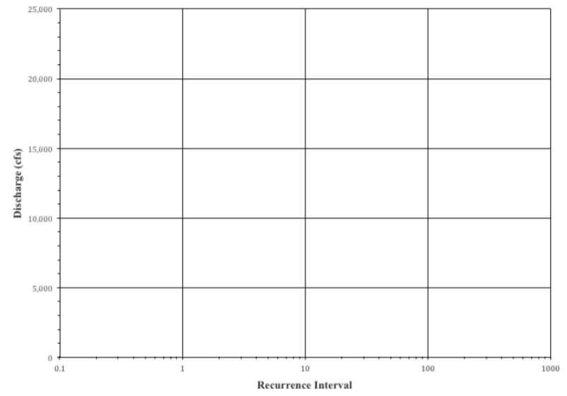
Now that you have completed the chart, plot the discharge against the recurrence interval on the following graph. Please note that the x-axis (for recurrence interval) is in logarithmic scale and you may need to estimate where the data points fall. A logarithmic scale is non-linear, based on orders of magnitude. Each mark on the x-axis is the previous mark multiplied by a value. Use a straight edge to draw a best fit line (a straight line along the graph that shows the general direction that the group of points seem to be heading – it doesn’t have to hit every point on the graph) through the graph when you are done, and then answer the following questions. Make sure your best fit line continues to the end of the graph.
12. On which date did a flood event have a recurrence interval of 0.5?
a. 2/27/2013 b. 10/13/2009 c. 3/10/2011 d. 4/20/2015
13. Of the following dated flood events, which one would you expect to happen more often?
a. 8/27/2008 b. 2/24/2013 c. 2/6/2010 d. 12/23/2013
14. Observe your best fit line. What approximate discharge would be associated with a 50-year recurrence interval?
a. 2,000 cfs b. 4,750 cfs c. 8,500 cfs d. 14,000 cfs
15. Flood stage, or bankfull stage, on Sweetwater Creek occurs at a discharge of ~4,500 cfs. According to your best fit line, what is the recurrence interval of such a discharge?
a. 0.5 years b. 3 years c. 25 years d. 50 years
16. During the flood event of 9/23/2009, the discharge measured at this gaging station was 21,200 cfs. Note where this would plot on your graph. Would the recurrence interval for this flood plot at:
a. 100 years b. 300 years c. 700 years d. longer than 1,000 years
17. Is it possible that a flood with a similar discharge to that of the event from 9/23/2009 could happen again in the next 20 years?
a. Yes b. No