6.3: Location and Focal Mechanisms
- Page ID
- 3549
\( \newcommand{\vecs}[1]{\overset { \scriptstyle \rightharpoonup} {\mathbf{#1}} } \)
\( \newcommand{\vecd}[1]{\overset{-\!-\!\rightharpoonup}{\vphantom{a}\smash {#1}}} \)
\( \newcommand{\id}{\mathrm{id}}\) \( \newcommand{\Span}{\mathrm{span}}\)
( \newcommand{\kernel}{\mathrm{null}\,}\) \( \newcommand{\range}{\mathrm{range}\,}\)
\( \newcommand{\RealPart}{\mathrm{Re}}\) \( \newcommand{\ImaginaryPart}{\mathrm{Im}}\)
\( \newcommand{\Argument}{\mathrm{Arg}}\) \( \newcommand{\norm}[1]{\| #1 \|}\)
\( \newcommand{\inner}[2]{\langle #1, #2 \rangle}\)
\( \newcommand{\Span}{\mathrm{span}}\)
\( \newcommand{\id}{\mathrm{id}}\)
\( \newcommand{\Span}{\mathrm{span}}\)
\( \newcommand{\kernel}{\mathrm{null}\,}\)
\( \newcommand{\range}{\mathrm{range}\,}\)
\( \newcommand{\RealPart}{\mathrm{Re}}\)
\( \newcommand{\ImaginaryPart}{\mathrm{Im}}\)
\( \newcommand{\Argument}{\mathrm{Arg}}\)
\( \newcommand{\norm}[1]{\| #1 \|}\)
\( \newcommand{\inner}[2]{\langle #1, #2 \rangle}\)
\( \newcommand{\Span}{\mathrm{span}}\) \( \newcommand{\AA}{\unicode[.8,0]{x212B}}\)
\( \newcommand{\vectorA}[1]{\vec{#1}} % arrow\)
\( \newcommand{\vectorAt}[1]{\vec{\text{#1}}} % arrow\)
\( \newcommand{\vectorB}[1]{\overset { \scriptstyle \rightharpoonup} {\mathbf{#1}} } \)
\( \newcommand{\vectorC}[1]{\textbf{#1}} \)
\( \newcommand{\vectorD}[1]{\overrightarrow{#1}} \)
\( \newcommand{\vectorDt}[1]{\overrightarrow{\text{#1}}} \)
\( \newcommand{\vectE}[1]{\overset{-\!-\!\rightharpoonup}{\vphantom{a}\smash{\mathbf {#1}}}} \)
\( \newcommand{\vecs}[1]{\overset { \scriptstyle \rightharpoonup} {\mathbf{#1}} } \)
\( \newcommand{\vecd}[1]{\overset{-\!-\!\rightharpoonup}{\vphantom{a}\smash {#1}}} \)
\(\newcommand{\avec}{\mathbf a}\) \(\newcommand{\bvec}{\mathbf b}\) \(\newcommand{\cvec}{\mathbf c}\) \(\newcommand{\dvec}{\mathbf d}\) \(\newcommand{\dtil}{\widetilde{\mathbf d}}\) \(\newcommand{\evec}{\mathbf e}\) \(\newcommand{\fvec}{\mathbf f}\) \(\newcommand{\nvec}{\mathbf n}\) \(\newcommand{\pvec}{\mathbf p}\) \(\newcommand{\qvec}{\mathbf q}\) \(\newcommand{\svec}{\mathbf s}\) \(\newcommand{\tvec}{\mathbf t}\) \(\newcommand{\uvec}{\mathbf u}\) \(\newcommand{\vvec}{\mathbf v}\) \(\newcommand{\wvec}{\mathbf w}\) \(\newcommand{\xvec}{\mathbf x}\) \(\newcommand{\yvec}{\mathbf y}\) \(\newcommand{\zvec}{\mathbf z}\) \(\newcommand{\rvec}{\mathbf r}\) \(\newcommand{\mvec}{\mathbf m}\) \(\newcommand{\zerovec}{\mathbf 0}\) \(\newcommand{\onevec}{\mathbf 1}\) \(\newcommand{\real}{\mathbb R}\) \(\newcommand{\twovec}[2]{\left[\begin{array}{r}#1 \\ #2 \end{array}\right]}\) \(\newcommand{\ctwovec}[2]{\left[\begin{array}{c}#1 \\ #2 \end{array}\right]}\) \(\newcommand{\threevec}[3]{\left[\begin{array}{r}#1 \\ #2 \\ #3 \end{array}\right]}\) \(\newcommand{\cthreevec}[3]{\left[\begin{array}{c}#1 \\ #2 \\ #3 \end{array}\right]}\) \(\newcommand{\fourvec}[4]{\left[\begin{array}{r}#1 \\ #2 \\ #3 \\ #4 \end{array}\right]}\) \(\newcommand{\cfourvec}[4]{\left[\begin{array}{c}#1 \\ #2 \\ #3 \\ #4 \end{array}\right]}\) \(\newcommand{\fivevec}[5]{\left[\begin{array}{r}#1 \\ #2 \\ #3 \\ #4 \\ #5 \\ \end{array}\right]}\) \(\newcommand{\cfivevec}[5]{\left[\begin{array}{c}#1 \\ #2 \\ #3 \\ #4 \\ #5 \\ \end{array}\right]}\) \(\newcommand{\mattwo}[4]{\left[\begin{array}{rr}#1 \amp #2 \\ #3 \amp #4 \\ \end{array}\right]}\) \(\newcommand{\laspan}[1]{\text{Span}\{#1\}}\) \(\newcommand{\bcal}{\cal B}\) \(\newcommand{\ccal}{\cal C}\) \(\newcommand{\scal}{\cal S}\) \(\newcommand{\wcal}{\cal W}\) \(\newcommand{\ecal}{\cal E}\) \(\newcommand{\coords}[2]{\left\{#1\right\}_{#2}}\) \(\newcommand{\gray}[1]{\color{gray}{#1}}\) \(\newcommand{\lgray}[1]{\color{lightgray}{#1}}\) \(\newcommand{\rank}{\operatorname{rank}}\) \(\newcommand{\row}{\text{Row}}\) \(\newcommand{\col}{\text{Col}}\) \(\renewcommand{\row}{\text{Row}}\) \(\newcommand{\nul}{\text{Nul}}\) \(\newcommand{\var}{\text{Var}}\) \(\newcommand{\corr}{\text{corr}}\) \(\newcommand{\len}[1]{\left|#1\right|}\) \(\newcommand{\bbar}{\overline{\bvec}}\) \(\newcommand{\bhat}{\widehat{\bvec}}\) \(\newcommand{\bperp}{\bvec^\perp}\) \(\newcommand{\xhat}{\widehat{\xvec}}\) \(\newcommand{\vhat}{\widehat{\vvec}}\) \(\newcommand{\uhat}{\widehat{\uvec}}\) \(\newcommand{\what}{\widehat{\wvec}}\) \(\newcommand{\Sighat}{\widehat{\Sigma}}\) \(\newcommand{\lt}{<}\) \(\newcommand{\gt}{>}\) \(\newcommand{\amp}{&}\) \(\definecolor{fillinmathshade}{gray}{0.9}\)When an earthquake occurs, how can we determine the location of the epicenter? The answer is that we can use the seismic waves themselves to tell us where they are coming from. The drawing below is a map showing the epicenter of an earthquake with several seismograph stations. Each seismograph station is at a different distance from the epicenter and records the seismic waves as they arrive at the station. The seismographs show that the time difference for the arrival of the P and S wave at each station is proportional to the distance of the station from epicenter.
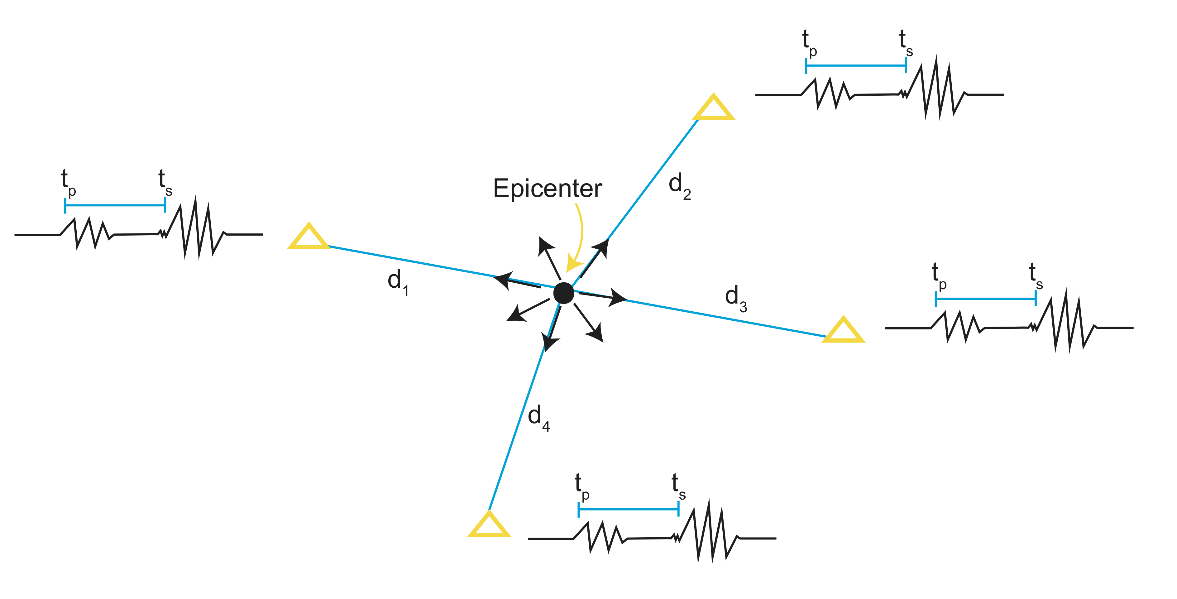
To find the epicenter of an earthquake there are four basic steps.
- Identify seismic wave phase arrival times at stations
- Calculate distance between individual stations and the epicenter
- Triangulate-use determined distances for multiple stations to locate epicenter
- Calculate origin time
Step 1 involves using the difference in arrival times of P and S waves that we talked about earlier. P and S waves travel the same distance, but have different arrival times. Thus, the distance in arrival time=difference in travel time.
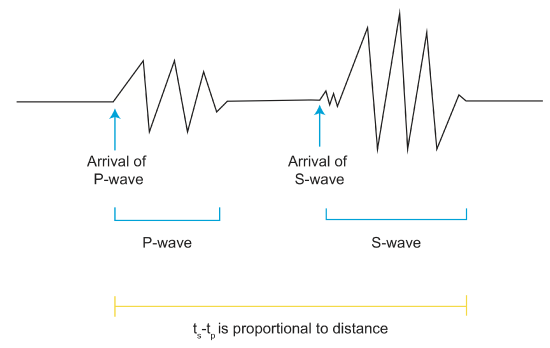
We can write a basic equation for distance traveled by starting with the equation: velocity=\(\frac{distance}{time}\). Rearrange and we get
\[d=tv\]
We know from experiments Vp, the P wave velocity, and Vs, the S wave velocity. We can also record on the seismograph tp and ts, the P and S wave travel times. We are thus trying to find x, the distance the waves traveled. For P waves:
\[x=v_pt_p\]
\[t_p=\frac{x}{v_p}\]
For S waves:
\[x=v_st_s\]
\[t_s=\frac{x}{v_s}\]
Using the difference in arrival times:
\[\begin{align} \Delta t &=t_p-t_s \\[4pt] &=\frac{x}{v_p}-\frac{x}{v_s} \\[4pt] &=x\left(\frac{1}{v_p}-\frac{1}{v_s}\right) \\[4pt] &=x\left(\frac{v_s}{v_sv_p}-\frac{v_p}{v_pv_s}\right) \\[4pt] &=x\left(\frac{v_s-v_p}{v_pv_s}\right) \end{align}\]
And finally
\[x=\Delta t \left[\frac{v_pv_s}{v_s-v_p}\right] \label{distance}\]
gives you the distance traveled.
Now that we know have the equation to find wave distance traveled, let's do a real example.
Example \(\PageIndex{1}\): Earthquake Location
Given that \(\Delta t=-10\, s\), \(v_p=5 \frac{km}{s}\), and \(v_s=3 \frac{km}{s}\), how far did the earthquake tarvel?
Solution
This is a simple application of Equation \ref{distance}.
\[\begin{align*} x &=\Delta t[\frac{v_pv_s}{v_s-v_p}] \\[4pt] &=-10[\frac{5\cdot 3}{3-5}] \\[4pt] &=-10[\frac{15}{-2}] \\[4pt] &=75\;km \end{align*}\]
Now we have the distance, but the earthquake could lie anywhere on a circle centered at that station with a radius=distance.
In order to find the exact location of the earthquake, we must repeat the distance calculation for at least two more stations. This will give us at least three circles with radius=distance, which we can cross reference as in the figure below.
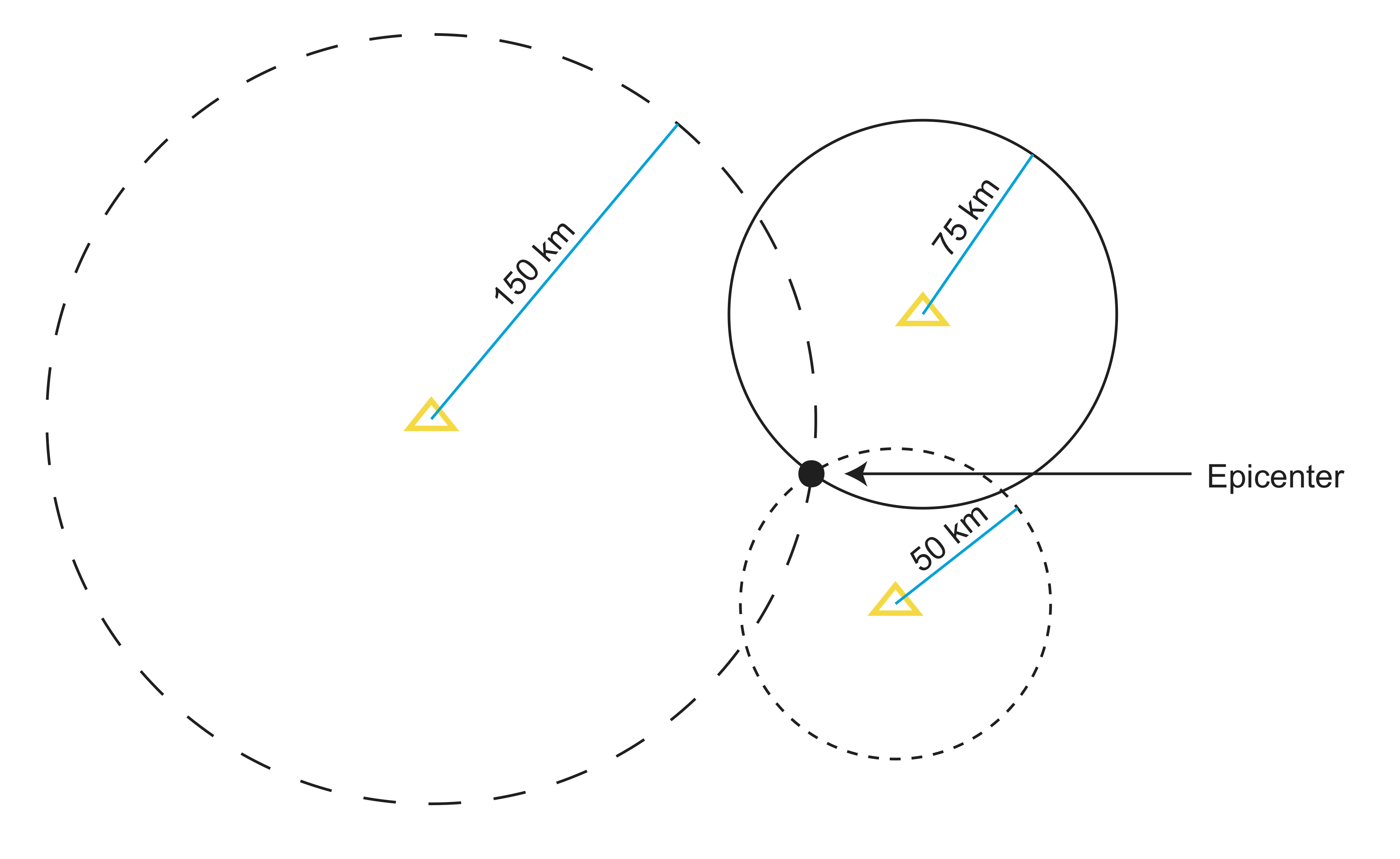
To locate the focus/hypocenter, you would need at least four stations to draw spheres in 3D in order to get depth.
Origin Time
We have now learned how to find: the arrival time, distance, velocity, and travel time. Now using those variables we can find the origin time.
\[origin\;time=arrival\;time-travel\;time\]
Example \(\PageIndex{2}\): Origin Time
Using the values we were given/calculated in the above example (vp=5\(\frac{km}{s}\), vs=3\(\frac{km}{s}\), and x=75 km), we can calculate the travel time:
\[\frac{75\; km}{5\;\frac{km}{s}}\]
\[15\;s\]
Note that the travel time can be calculated with any station and both P and S wave arrivals.
If we know that the arrival time was at 11:30:45 (11:30 and 45 sec), the origin time=11:30:45-00:00:15. Thus the origin time is 11:30:30.
Focal Mechanisms
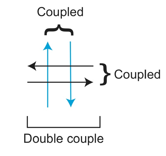
Focal mechanisms give information about the type of deformation in the source region that generates the seismic waves. In other words, focal mechanisms show a simple seismic model of faulting. They are also a 'moment tensor' or 'beach ball diagram'. A moment tensor is like a stress tensor, it gives you the state of stress. Focal mechanisms are a double representation of slip, this refers to the coupling of forces, like in Figure \(\PageIndex{4}\).
Slip on a fault also causes volumetric changes. Look at the figure below to better understand this.
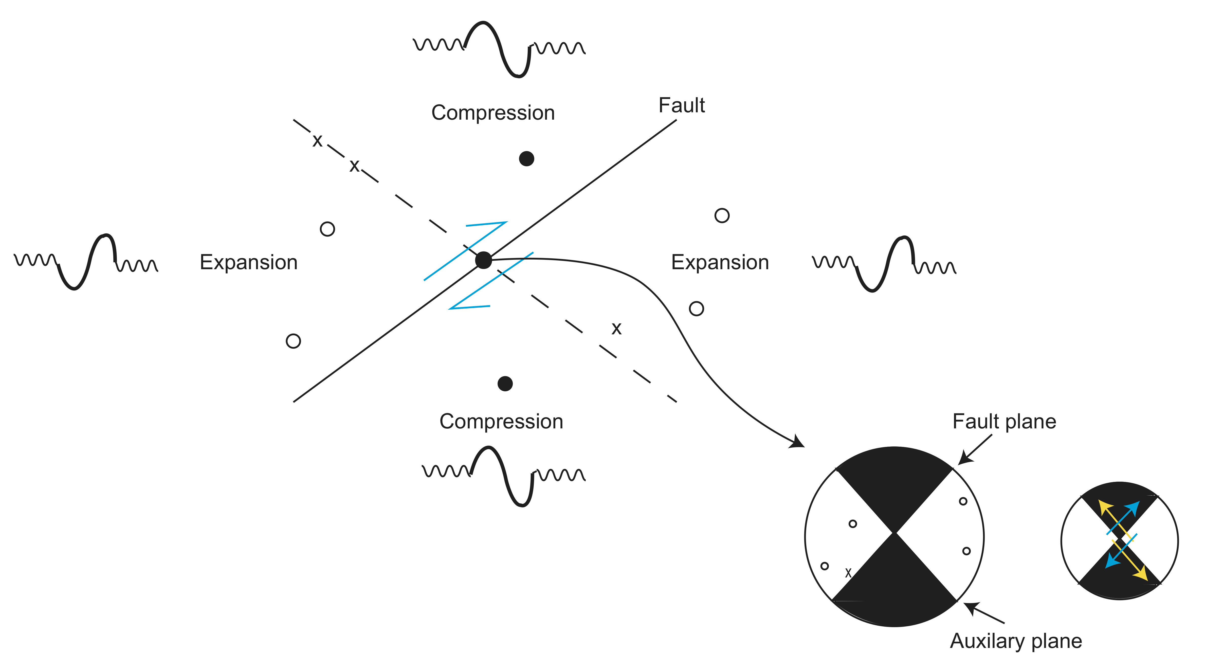
The first motion of the fault that causes the volumetric changes is the P waves that are recorded at stations. The various motions of the fault are represented on what is known as a beach ball. The regions of compression indicate a first motion of up  and are represented by a closed dot \(\bullet\). The regions of expansion
  indicate a first motion of down and are represented by an open dot \(\circ\). If there is no detected signal,
  this is represented by an \(\times\). All together, the motions of the fault look like the figure below.
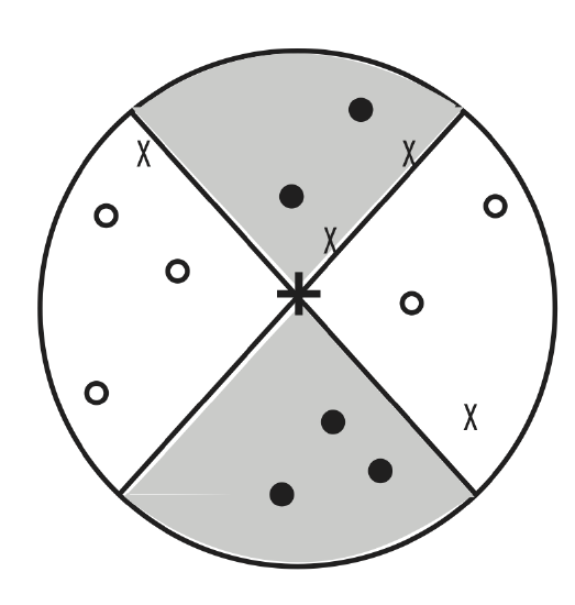
To combine all of the data into a cohesive picture of fault motion, we will use a beach ball. A basic beach ball is seen below.

Visualizing fault planes on a sphere is often difficult, so let's look at it from some different angles.
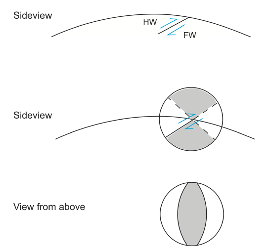
When drawing a beach ball, we must ensure that the auxiliary plane is perpendicular to the fault plane. Remember that the fault plane is where displacement occurs. These two planes are also called nodal planes.
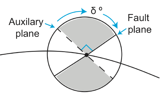
There are three principal axes on a beach ball, the N axis, P axis, and T axis. These axes are all orthogonal to each other.
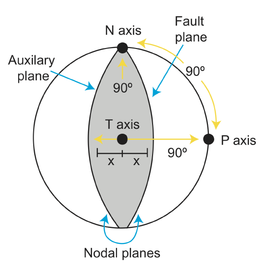
Figure \(\PageIndex{10}\): 3 Principal Axes
The N axis, also called the b axis, is the null axis. It is the intersection of the two nodal planes. The P axis is the pressure axis. It bisects the angle between the nodal planes, and has the largest amplitude down first motion. The T axis is the tension axis. It also bisects the angle between the nodal planes, and has the largest amplitude up first motion.
To get a better understanding of a how different fault types are modeled on a beach ball:

How do you determine which nodal plane is the fault plane?
- Look at the geology
- Look at the aftershock pattern
FIGURE Magali will make figure for use
Summary
That was a lot of new information to cover in one section. Here are some quick glance takeaways of focal mechanisms can tell you:
- Approximate strike of fault
- What type of faulting occurred
- Overall sense of motion in a region
- Regions of compression and tension


