5.4: Seismic Reflection (Single Layer)
- Page ID
- 3541
\( \newcommand{\vecs}[1]{\overset { \scriptstyle \rightharpoonup} {\mathbf{#1}} } \)
\( \newcommand{\vecd}[1]{\overset{-\!-\!\rightharpoonup}{\vphantom{a}\smash {#1}}} \)
\( \newcommand{\id}{\mathrm{id}}\) \( \newcommand{\Span}{\mathrm{span}}\)
( \newcommand{\kernel}{\mathrm{null}\,}\) \( \newcommand{\range}{\mathrm{range}\,}\)
\( \newcommand{\RealPart}{\mathrm{Re}}\) \( \newcommand{\ImaginaryPart}{\mathrm{Im}}\)
\( \newcommand{\Argument}{\mathrm{Arg}}\) \( \newcommand{\norm}[1]{\| #1 \|}\)
\( \newcommand{\inner}[2]{\langle #1, #2 \rangle}\)
\( \newcommand{\Span}{\mathrm{span}}\)
\( \newcommand{\id}{\mathrm{id}}\)
\( \newcommand{\Span}{\mathrm{span}}\)
\( \newcommand{\kernel}{\mathrm{null}\,}\)
\( \newcommand{\range}{\mathrm{range}\,}\)
\( \newcommand{\RealPart}{\mathrm{Re}}\)
\( \newcommand{\ImaginaryPart}{\mathrm{Im}}\)
\( \newcommand{\Argument}{\mathrm{Arg}}\)
\( \newcommand{\norm}[1]{\| #1 \|}\)
\( \newcommand{\inner}[2]{\langle #1, #2 \rangle}\)
\( \newcommand{\Span}{\mathrm{span}}\) \( \newcommand{\AA}{\unicode[.8,0]{x212B}}\)
\( \newcommand{\vectorA}[1]{\vec{#1}} % arrow\)
\( \newcommand{\vectorAt}[1]{\vec{\text{#1}}} % arrow\)
\( \newcommand{\vectorB}[1]{\overset { \scriptstyle \rightharpoonup} {\mathbf{#1}} } \)
\( \newcommand{\vectorC}[1]{\textbf{#1}} \)
\( \newcommand{\vectorD}[1]{\overrightarrow{#1}} \)
\( \newcommand{\vectorDt}[1]{\overrightarrow{\text{#1}}} \)
\( \newcommand{\vectE}[1]{\overset{-\!-\!\rightharpoonup}{\vphantom{a}\smash{\mathbf {#1}}}} \)
\( \newcommand{\vecs}[1]{\overset { \scriptstyle \rightharpoonup} {\mathbf{#1}} } \)
\( \newcommand{\vecd}[1]{\overset{-\!-\!\rightharpoonup}{\vphantom{a}\smash {#1}}} \)
\(\newcommand{\avec}{\mathbf a}\) \(\newcommand{\bvec}{\mathbf b}\) \(\newcommand{\cvec}{\mathbf c}\) \(\newcommand{\dvec}{\mathbf d}\) \(\newcommand{\dtil}{\widetilde{\mathbf d}}\) \(\newcommand{\evec}{\mathbf e}\) \(\newcommand{\fvec}{\mathbf f}\) \(\newcommand{\nvec}{\mathbf n}\) \(\newcommand{\pvec}{\mathbf p}\) \(\newcommand{\qvec}{\mathbf q}\) \(\newcommand{\svec}{\mathbf s}\) \(\newcommand{\tvec}{\mathbf t}\) \(\newcommand{\uvec}{\mathbf u}\) \(\newcommand{\vvec}{\mathbf v}\) \(\newcommand{\wvec}{\mathbf w}\) \(\newcommand{\xvec}{\mathbf x}\) \(\newcommand{\yvec}{\mathbf y}\) \(\newcommand{\zvec}{\mathbf z}\) \(\newcommand{\rvec}{\mathbf r}\) \(\newcommand{\mvec}{\mathbf m}\) \(\newcommand{\zerovec}{\mathbf 0}\) \(\newcommand{\onevec}{\mathbf 1}\) \(\newcommand{\real}{\mathbb R}\) \(\newcommand{\twovec}[2]{\left[\begin{array}{r}#1 \\ #2 \end{array}\right]}\) \(\newcommand{\ctwovec}[2]{\left[\begin{array}{c}#1 \\ #2 \end{array}\right]}\) \(\newcommand{\threevec}[3]{\left[\begin{array}{r}#1 \\ #2 \\ #3 \end{array}\right]}\) \(\newcommand{\cthreevec}[3]{\left[\begin{array}{c}#1 \\ #2 \\ #3 \end{array}\right]}\) \(\newcommand{\fourvec}[4]{\left[\begin{array}{r}#1 \\ #2 \\ #3 \\ #4 \end{array}\right]}\) \(\newcommand{\cfourvec}[4]{\left[\begin{array}{c}#1 \\ #2 \\ #3 \\ #4 \end{array}\right]}\) \(\newcommand{\fivevec}[5]{\left[\begin{array}{r}#1 \\ #2 \\ #3 \\ #4 \\ #5 \\ \end{array}\right]}\) \(\newcommand{\cfivevec}[5]{\left[\begin{array}{c}#1 \\ #2 \\ #3 \\ #4 \\ #5 \\ \end{array}\right]}\) \(\newcommand{\mattwo}[4]{\left[\begin{array}{rr}#1 \amp #2 \\ #3 \amp #4 \\ \end{array}\right]}\) \(\newcommand{\laspan}[1]{\text{Span}\{#1\}}\) \(\newcommand{\bcal}{\cal B}\) \(\newcommand{\ccal}{\cal C}\) \(\newcommand{\scal}{\cal S}\) \(\newcommand{\wcal}{\cal W}\) \(\newcommand{\ecal}{\cal E}\) \(\newcommand{\coords}[2]{\left\{#1\right\}_{#2}}\) \(\newcommand{\gray}[1]{\color{gray}{#1}}\) \(\newcommand{\lgray}[1]{\color{lightgray}{#1}}\) \(\newcommand{\rank}{\operatorname{rank}}\) \(\newcommand{\row}{\text{Row}}\) \(\newcommand{\col}{\text{Col}}\) \(\renewcommand{\row}{\text{Row}}\) \(\newcommand{\nul}{\text{Nul}}\) \(\newcommand{\var}{\text{Var}}\) \(\newcommand{\corr}{\text{corr}}\) \(\newcommand{\len}[1]{\left|#1\right|}\) \(\newcommand{\bbar}{\overline{\bvec}}\) \(\newcommand{\bhat}{\widehat{\bvec}}\) \(\newcommand{\bperp}{\bvec^\perp}\) \(\newcommand{\xhat}{\widehat{\xvec}}\) \(\newcommand{\vhat}{\widehat{\vvec}}\) \(\newcommand{\uhat}{\widehat{\uvec}}\) \(\newcommand{\what}{\widehat{\wvec}}\) \(\newcommand{\Sighat}{\widehat{\Sigma}}\) \(\newcommand{\lt}{<}\) \(\newcommand{\gt}{>}\) \(\newcommand{\amp}{&}\) \(\definecolor{fillinmathshade}{gray}{0.9}\)Reflection surveys follow the same basic principles as refraction surveys, except of course they use reflected waves instead of refracted waves. We can use reflected waves to get h and v1, but we cannot get v2 unless we have a reflection from a deeper layer.
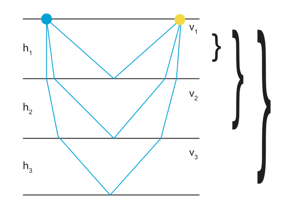
If there are multiple layers, we can determine each layers data such as height and velocity by working down one layer at a time. However, today we will only focus on a single layer subsurface. We can use the layer geometry to get a travel-time equation.
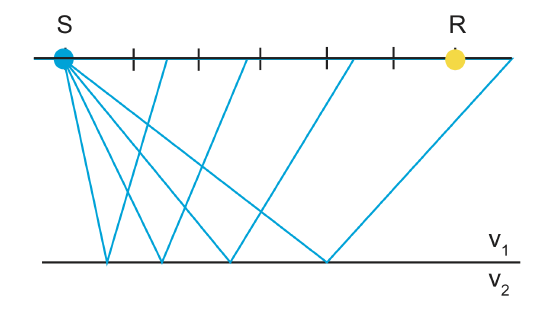
In the case of reflection, we can have v2>v1 or v2<v1, we will get a reflected wave either way.
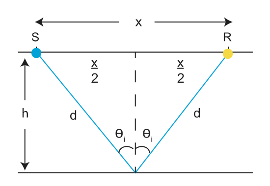
Starting with our distance equation,
\[d=v\cdot t\]
\[t=\frac{d}{v}\]
\[d^2=(\frac{x}{2})^2+h^2\]
The total distance a reflected wave will travel is 2d, because the wave must go down and then back up to the receiver.
\[2d=2((\frac{x}{2})^2+h^2)^{\frac{1}{2}}\]
\[2d=(x^2+4h^2)^{\frac{1}{2}}\]
\[t=\frac{2d}{v_1}\]
\[t=\frac{\sqrt{x^2+4h^2}}{v_1}\]
What is the intercept time?
t(x=0)=to=\(\frac{2h}{v_1}\)
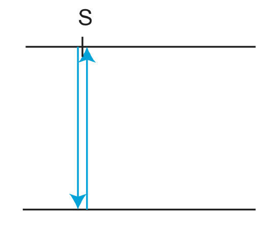
For a vertically reflected wave, if you know v1, you can get h.
\[h=\frac{v_1t_o}{2}\]
We've just said that calculating h from a vertically reflected wave is easy if you know v1. So how do we get v1? We are going to assume that we can't measure the direct wave (this is not usually true for layer 1, but definitely true for deeper layers-there is no direct wave here).
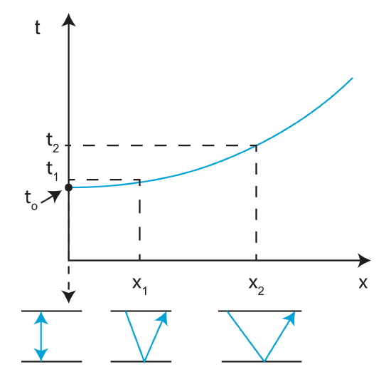
From the last section, we know that the graph of a refracted wave is a line. So what is the shape of t(x) for a reflected wave?
Figure \(\PageIndex{4}\): Vertically Reflected Wave
\[t^2=\frac{x^2}{v_1^2}+\frac{4h^2}{v_1^2}\]
We know that \(\frac{4h^2}{v_1^2}\) can also be written as to2.
\[t_o^2=t^2-\frac{x^2}{v_1^2}\]
\[1=\frac{t^2}{t_o^2}-\frac{x^2}{v_1^2t_o^2}\]
The above equation is the equation for a hyperbola where a=to and b=v1to. The intercept is at to. The slope at large x=\(\frac{a}{b}=\frac{t_o}{v_1t_o}=\frac{1}{v_1}\).
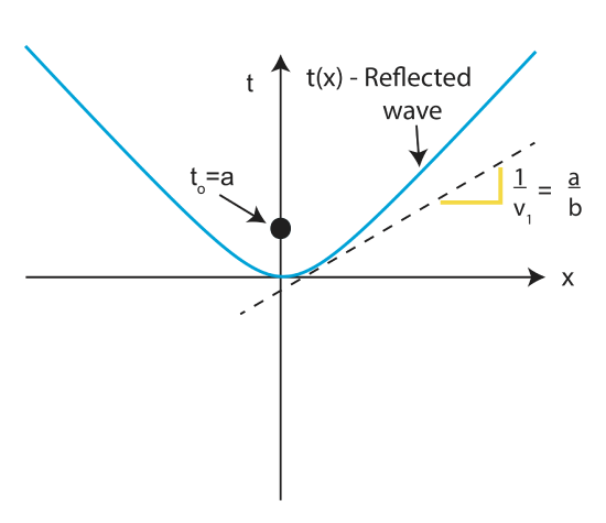
We can derive that the equation for to is:
\[t_o=\frac{2h}{v_1}\]
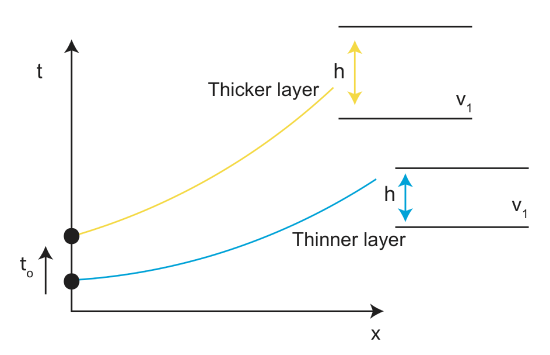
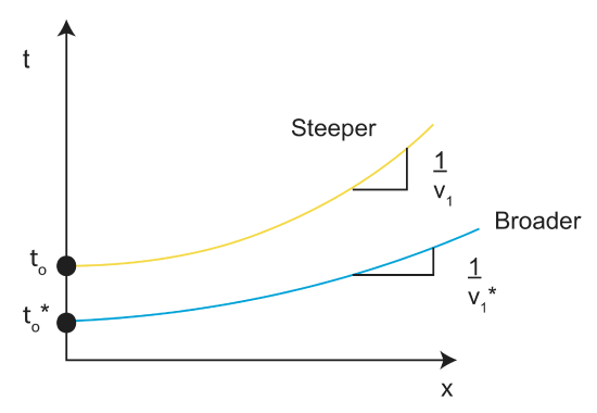
The figure below shows how the hyperbola changes with layer thickness. The hyperbola will increase with increasing layer thickness.
What if two layers have the same thickness but different velocities?
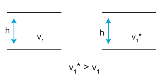
In the above figure, v1*>v1. Using our equation \(t_o=\frac{2h}{v_1}\), to\(\downarrow\) for v1\(\uparrow\). Since the slope of the hyperbola \(\frac{a}{b}\) is \(\frac{1}{v_1}\), we can see that as v1 increases, we will get a lower slope (a broader shape).
In the case of multiple layers, the travel time equation is also a hyperbola. We just used a single layer example to understand the basic concepts. Now that we have a basic understanding of the different terms and how the data can be graphed, we are going to analyze it using a method called Normal Move-out (NMO).
\[T_{NMO}=t(x)-t_o\]
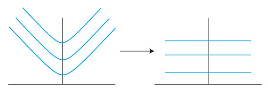
The equation for TNMO gives us the "shape of the hyperbola". If we could correct for NMO, all reflections would look like they come from a vertical reflection. As you 'move-out' along the hyperbola, the path the ray takes gets longer and longer. Thus by correcting for NMO, we are looking at data close to the first few recievers, ie those that have taken shorter paths and have not 'moved-out'.
At small x, we can approximate
\[t(x)\approx t_o+\frac{x}{2v_1^2t_o}\]
and that
\[t(x)^2=t_o^2+\frac{x^2}{v_1^2}\]
Using binomial expansion, we get that
\[t(x)=t_o(1+(\frac{x^2}{v_1t_o})^2)^{\frac{1}{2}}\]
then
\[T_{NMO}=t(x)-t_o\]
Substituting for t(x):
\[T_{NMO}\approx\frac{x^2}{2v_1^2t_o}\]
Solve for v1
\[v_1\approx\frac{x}{\sqrt{2t_oT_{NMO}}}\]
When you are actually analyzing a travel time graph, there are several steps you can take to get information on the subsurface.
- Measure (or read off) to, t(x), and x
- If x has a small value, calculate TNMO=t(x)-to
- Calculate \(v_1\approx\frac{x}{\sqrt{2t_oT_{NMO}}}\)
- Calculate \(h=\frac{v_1t_o}{2}\)
For real processing of reflection data
- We guess v1 and h
- Calculate predicted NMO
- Correct arrivals
- Are they flat? If not, try new values (loop through many values and find peak sum)
