3.4: Isostasy
- Page ID
- 3522
\( \newcommand{\vecs}[1]{\overset { \scriptstyle \rightharpoonup} {\mathbf{#1}} } \)
\( \newcommand{\vecd}[1]{\overset{-\!-\!\rightharpoonup}{\vphantom{a}\smash {#1}}} \)
\( \newcommand{\id}{\mathrm{id}}\) \( \newcommand{\Span}{\mathrm{span}}\)
( \newcommand{\kernel}{\mathrm{null}\,}\) \( \newcommand{\range}{\mathrm{range}\,}\)
\( \newcommand{\RealPart}{\mathrm{Re}}\) \( \newcommand{\ImaginaryPart}{\mathrm{Im}}\)
\( \newcommand{\Argument}{\mathrm{Arg}}\) \( \newcommand{\norm}[1]{\| #1 \|}\)
\( \newcommand{\inner}[2]{\langle #1, #2 \rangle}\)
\( \newcommand{\Span}{\mathrm{span}}\)
\( \newcommand{\id}{\mathrm{id}}\)
\( \newcommand{\Span}{\mathrm{span}}\)
\( \newcommand{\kernel}{\mathrm{null}\,}\)
\( \newcommand{\range}{\mathrm{range}\,}\)
\( \newcommand{\RealPart}{\mathrm{Re}}\)
\( \newcommand{\ImaginaryPart}{\mathrm{Im}}\)
\( \newcommand{\Argument}{\mathrm{Arg}}\)
\( \newcommand{\norm}[1]{\| #1 \|}\)
\( \newcommand{\inner}[2]{\langle #1, #2 \rangle}\)
\( \newcommand{\Span}{\mathrm{span}}\) \( \newcommand{\AA}{\unicode[.8,0]{x212B}}\)
\( \newcommand{\vectorA}[1]{\vec{#1}} % arrow\)
\( \newcommand{\vectorAt}[1]{\vec{\text{#1}}} % arrow\)
\( \newcommand{\vectorB}[1]{\overset { \scriptstyle \rightharpoonup} {\mathbf{#1}} } \)
\( \newcommand{\vectorC}[1]{\textbf{#1}} \)
\( \newcommand{\vectorD}[1]{\overrightarrow{#1}} \)
\( \newcommand{\vectorDt}[1]{\overrightarrow{\text{#1}}} \)
\( \newcommand{\vectE}[1]{\overset{-\!-\!\rightharpoonup}{\vphantom{a}\smash{\mathbf {#1}}}} \)
\( \newcommand{\vecs}[1]{\overset { \scriptstyle \rightharpoonup} {\mathbf{#1}} } \)
\( \newcommand{\vecd}[1]{\overset{-\!-\!\rightharpoonup}{\vphantom{a}\smash {#1}}} \)
\(\newcommand{\avec}{\mathbf a}\) \(\newcommand{\bvec}{\mathbf b}\) \(\newcommand{\cvec}{\mathbf c}\) \(\newcommand{\dvec}{\mathbf d}\) \(\newcommand{\dtil}{\widetilde{\mathbf d}}\) \(\newcommand{\evec}{\mathbf e}\) \(\newcommand{\fvec}{\mathbf f}\) \(\newcommand{\nvec}{\mathbf n}\) \(\newcommand{\pvec}{\mathbf p}\) \(\newcommand{\qvec}{\mathbf q}\) \(\newcommand{\svec}{\mathbf s}\) \(\newcommand{\tvec}{\mathbf t}\) \(\newcommand{\uvec}{\mathbf u}\) \(\newcommand{\vvec}{\mathbf v}\) \(\newcommand{\wvec}{\mathbf w}\) \(\newcommand{\xvec}{\mathbf x}\) \(\newcommand{\yvec}{\mathbf y}\) \(\newcommand{\zvec}{\mathbf z}\) \(\newcommand{\rvec}{\mathbf r}\) \(\newcommand{\mvec}{\mathbf m}\) \(\newcommand{\zerovec}{\mathbf 0}\) \(\newcommand{\onevec}{\mathbf 1}\) \(\newcommand{\real}{\mathbb R}\) \(\newcommand{\twovec}[2]{\left[\begin{array}{r}#1 \\ #2 \end{array}\right]}\) \(\newcommand{\ctwovec}[2]{\left[\begin{array}{c}#1 \\ #2 \end{array}\right]}\) \(\newcommand{\threevec}[3]{\left[\begin{array}{r}#1 \\ #2 \\ #3 \end{array}\right]}\) \(\newcommand{\cthreevec}[3]{\left[\begin{array}{c}#1 \\ #2 \\ #3 \end{array}\right]}\) \(\newcommand{\fourvec}[4]{\left[\begin{array}{r}#1 \\ #2 \\ #3 \\ #4 \end{array}\right]}\) \(\newcommand{\cfourvec}[4]{\left[\begin{array}{c}#1 \\ #2 \\ #3 \\ #4 \end{array}\right]}\) \(\newcommand{\fivevec}[5]{\left[\begin{array}{r}#1 \\ #2 \\ #3 \\ #4 \\ #5 \\ \end{array}\right]}\) \(\newcommand{\cfivevec}[5]{\left[\begin{array}{c}#1 \\ #2 \\ #3 \\ #4 \\ #5 \\ \end{array}\right]}\) \(\newcommand{\mattwo}[4]{\left[\begin{array}{rr}#1 \amp #2 \\ #3 \amp #4 \\ \end{array}\right]}\) \(\newcommand{\laspan}[1]{\text{Span}\{#1\}}\) \(\newcommand{\bcal}{\cal B}\) \(\newcommand{\ccal}{\cal C}\) \(\newcommand{\scal}{\cal S}\) \(\newcommand{\wcal}{\cal W}\) \(\newcommand{\ecal}{\cal E}\) \(\newcommand{\coords}[2]{\left\{#1\right\}_{#2}}\) \(\newcommand{\gray}[1]{\color{gray}{#1}}\) \(\newcommand{\lgray}[1]{\color{lightgray}{#1}}\) \(\newcommand{\rank}{\operatorname{rank}}\) \(\newcommand{\row}{\text{Row}}\) \(\newcommand{\col}{\text{Col}}\) \(\renewcommand{\row}{\text{Row}}\) \(\newcommand{\nul}{\text{Nul}}\) \(\newcommand{\var}{\text{Var}}\) \(\newcommand{\corr}{\text{corr}}\) \(\newcommand{\len}[1]{\left|#1\right|}\) \(\newcommand{\bbar}{\overline{\bvec}}\) \(\newcommand{\bhat}{\widehat{\bvec}}\) \(\newcommand{\bperp}{\bvec^\perp}\) \(\newcommand{\xhat}{\widehat{\xvec}}\) \(\newcommand{\vhat}{\widehat{\vvec}}\) \(\newcommand{\uhat}{\widehat{\uvec}}\) \(\newcommand{\what}{\widehat{\wvec}}\) \(\newcommand{\Sighat}{\widehat{\Sigma}}\) \(\newcommand{\lt}{<}\) \(\newcommand{\gt}{>}\) \(\newcommand{\amp}{&}\) \(\definecolor{fillinmathshade}{gray}{0.9}\)Very broad or long wave-length topography is more likely to be compensated than smaller scale topography. This is because large topography is more massive and causes the lithosphere to bend into the deeper viscous mantle. Smaller topographic features can be supported by the strength of the lithosphere, and therefore no compensating mass anomaly forms beneath the topography.
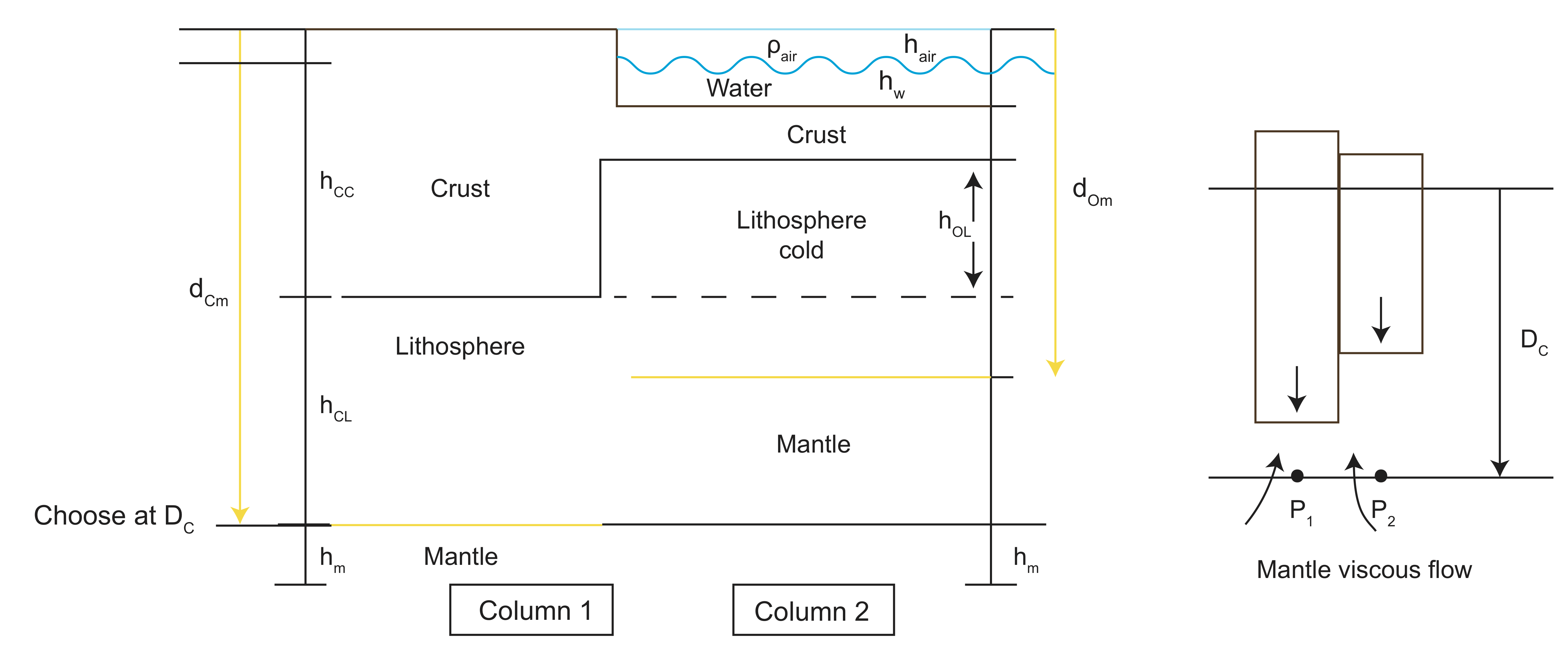
Compensated topography is also referred as isostatically compensated topography, where the word isostatic refers to equal pressure (or stress) in the viscous lithosphere or mantle beneath adjacent columns of static (not moving up or down, or moving very, very slowly) mass. In Figure \(\PageIndex{2}\), the pressures, \(P_1\) and \(P_2\) are equal at a depth, \(D_c\), called the depth of compensation. Beneath \(D_c\) there are no differences in the density structure of the two columns.
\[P=\sum_{i=1}^{n}\rho_ih_ig\]
The concept of isostasy is used to understand why the average height of one region of a plate is different than another region of plate.
Start with familiar concept: ice floating in water.
- Thicker ice floats higher than thinner ice because its mass is less.
- However, there is also much more ice beneath the water line than above the water line because,
- the density difference between ice and water is smaller than the density difference between ice and air.
Consider a continent ocean system:
- Two adjacent columns of mass: continental and oceanic
- The pressure in the viscous (flowing) layer at the bottom is due to the weight (\(\sum\rho g h\) of the column above.
- In isostatic equilibrium, the pressure at the bottom of each column (below where there are any differences in the density) is the same in both columns (\(P_1 = P_2\)
- Write out the sum for the pressure in each column (this reduces to the sum of the density times the thickness in each layer)
- Set the pressures equal.
- This equation can be used to determine the height difference between the two columns or the difference in the thickness of the crust extending into the viscous lithosphere.
- However, a second equation is needed, otherwise there are two unknowns.
- The second equation comes from equating the heights. Then one of the unknowns can be solved for and this equation is substituted into the pressure balance equation.

Isostasy Problem Recipe:
The approach to any isostasy problem is the same
- Draw a picture
- Determine \(D_c\) as the depth where there are no more differences in density between the two columns
- Write down the equation \(P_1=P_2\)
- Simplify: cancel\(g\)'s and combine like terms
- Write down \( \sum H_{1i} = \sum H_{2i} \) and use this to get rid of extra unknowns (solve for the unknown you don't want to know)
- Solve for desired unknown
Example relative Height of Continent and Oceans
Why is the average elevation of continents higher than the average height of oceans?
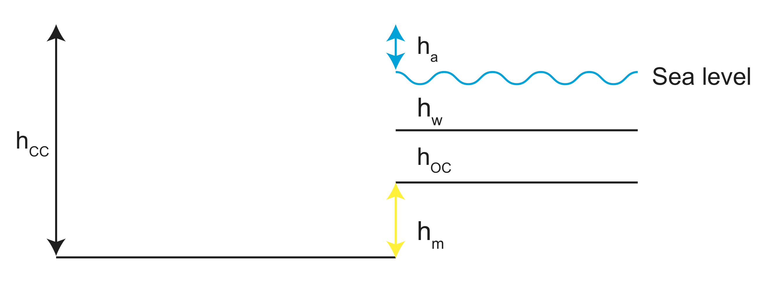
Assume that we know all the densities in the problem, and we know the crustal thicknesses (\(h_{cc} and h_{oc}\) and the thickness of the water layer \(h_w\).
From the drawing we see that we can take the depth of compensation at the base of the continent because below this depth there are no differences in density between the to two columes
First, we write out the sums of pressure for both columns and set them equal:
\[\rho_{cc}h_{cc}g =\rho_{air}h_{air}g + \rho_{w}h_{w}g + \rho_{oc}h_{oc}g + \rho_{L}h_{L}g \label{ex1}\]
(here I have used the subscript \(L\) instead of \(oL\) for the thickness and density of the lithosphere mantle in the oceanic column.
Next we can cancel all g's, and Equation \ref{ex1} now reads:\[\rho_{cc}h_{cc} = \rho_{air}h_{air} + \rho_{w}h_{w} + \rho_{oc}h_{oc} + \rho_{L}h_{L}\]
We can now see that we have 2 unknowns, \(h_{air}\) and \(h_L\) and thus we will need a second equation. The total thickness of the crust is equal to the sum of the thicknesses in the oceanic column:
\[h_{cc}=h_{air} + h_{w} + h_{oc} + h_{L}\]
We solve this equation to for \(h_L\) because we don't know it and do not want to know it (we want to know \(h_{air}\)):
\[h_{L}=h_{cc} - h_{air} - h_{w} - h_{oc}\]
Now substitute the equation above for \(h_L\) into the pressure balance equation. This removes \(h_L\) from the equation allowing you to solve for hair:
\[ \rho_{cc}h_{cc} = \rho_{air}h_{air} + \rho_{w}h_{w} + \rho_{oc}h_{oc} + \rho_{L}h_{cc} - \rho_{L}h_{air} - \rho_{L}h_{w} - \rho_{L}h_{oc} \]
Note that now you have three negative terms that all depend on \(\rho_L\) but have different thicknesses. The next step is to combine these terms with the positive terms that have the same thickness.
Combine the "like terms", that is combine the terms that have the same thickness (keeping \(h_a\) on the left-hand side)
\[ 0 = + h_{cc}(\rho_L - \rho_{cc}) - h_a(\rho_L -\rho_a) - h_w(\rho_L - \rho_w) - h_{oc}(\rho_L - \rho_{oc}) \]
Note that, for the last three terms we have taken a negative sign out front so the density difference is a positive number.
Next, re-arrange by adding the negative \(h_a\) term to the other side
\[h_a(\rho_L-\rho_a) = (\rho_L - \rho_{cc})h_{cc} - h_w(\rho_L-\rho_w)- h_{oc}(\rho_L-\rho_{oc}) \]
Finally divide \( (\rho_L-\rho_a) \) to get \(h_a\) alone:
\[ h_a=h_{cc}\left(\frac{\rho_L-\rho_{cc}}{\rho_L-\rho_a}\right)-h_w \left(\frac{\rho_L-\rho_w}{\rho_L-\rho_a}\right) -h_{oc}\left(\frac{\rho_L-\rho_{oc}}{\rho_L-\rho_a}\right)\]
Note that all terms on the right are fractional heights weighted by the density difference across each layer relative to the density different between the air and the continental crust. This is the outcome of every isostatic balance problem an illustrates how the pressure balance is achieved for each layer.
Example Time Changes

At some time T1 the height of mountain range above sea level is \(h_{a1}\) and the thickness of the crust is \(h_{cc}\). After erosion at time T2 the thickness of the crust is smaller by \(\Delta h\). Because there is no less mass weighting the continent down it will rise buoyantly (like removing weight from a floating ship). What is the height of the mountain range at time \(T_2\) (assuming isostatic balance).
First, let's consider what stays the same: the thickness of the water hw and the oceanic crust \(h_{oc}\)
Second, what changes? Both the height of the continent above sea-level \(h_a\) and the thickness of the mantle root \(h_m\) change.
Start by writing the isostatic balance for time \(T_1\) using the solution given above in the previous example:
\[h_{a1} = h_{cc}\left(\frac{\rho_L-\rho_{cc}}{\rho_L-\rho_a}\right) - h_w \left(\frac{\rho_L-\rho_w}{\rho_L-\rho_a}\right) -h_{oc}\left(\frac{\rho_L-\rho_{oc}}{\rho_L-\rho_a}\right)\]
Now, let \( A_1 = - h_w(\frac{\rho_L-\rho_{w}}{\rho_L-\rho_a})\) and \(A_2 = - h_{oc}(\frac{\rho_L-\rho_{oc}}{\rho_L-\rho_a})\). These terms do not change between time 1 and time 2 because \(h_w\) and \(h_{oc}\) do not change.
Next, write the equation for the height of the continent at time \(T_2\):
\[h_{a2}=(h_{cc} - \Delta h)(\frac{\rho_L-\rho_{cc}}{\rho_L-\rho_a}) + A_1 + A_2\]
Expand the first term
\[h_{a2}= \left(h_{cc}(\frac{\rho_L-\rho_{cc}}{\rho_L-\rho_a})+A_1+A_2 \right) - \Delta h(\frac{\rho_L-\rho_{cc}}{\rho_L-\rho_a})\]
Now note that the first three terms are equal to where \(h_{a1}\).
\[h_{a2}=h_{a1} - \Delta h(\frac{\rho_L-\rho_{cc}}{\rho_L-\rho_a})\]
So the final height of the continent after erosion is equal to original height, minus a density weighted fraction of the thickness that was eroded. The density fraction is less than 1, so change in height is less than \(\Delta h\). The reason is that the continent moves up a little bit in response to the removal of mass by erosion.
Example Depth of an Ocean Basin
Mid ocean ridge are usually found at depths of about 2500 m (2.5 km) below sea level. As the oceanic plate moves away from the mid ocean ridge, the lithosphere cools becoming thicker. Because colder rock has a higher density than warmer rock this thickening lithosphere increases the weight of the tectonic plate, and so it sinks into mantle. By the time the lithosphere reaches 80 My years old, the ocean depth is more like 4500 to 5000 m.
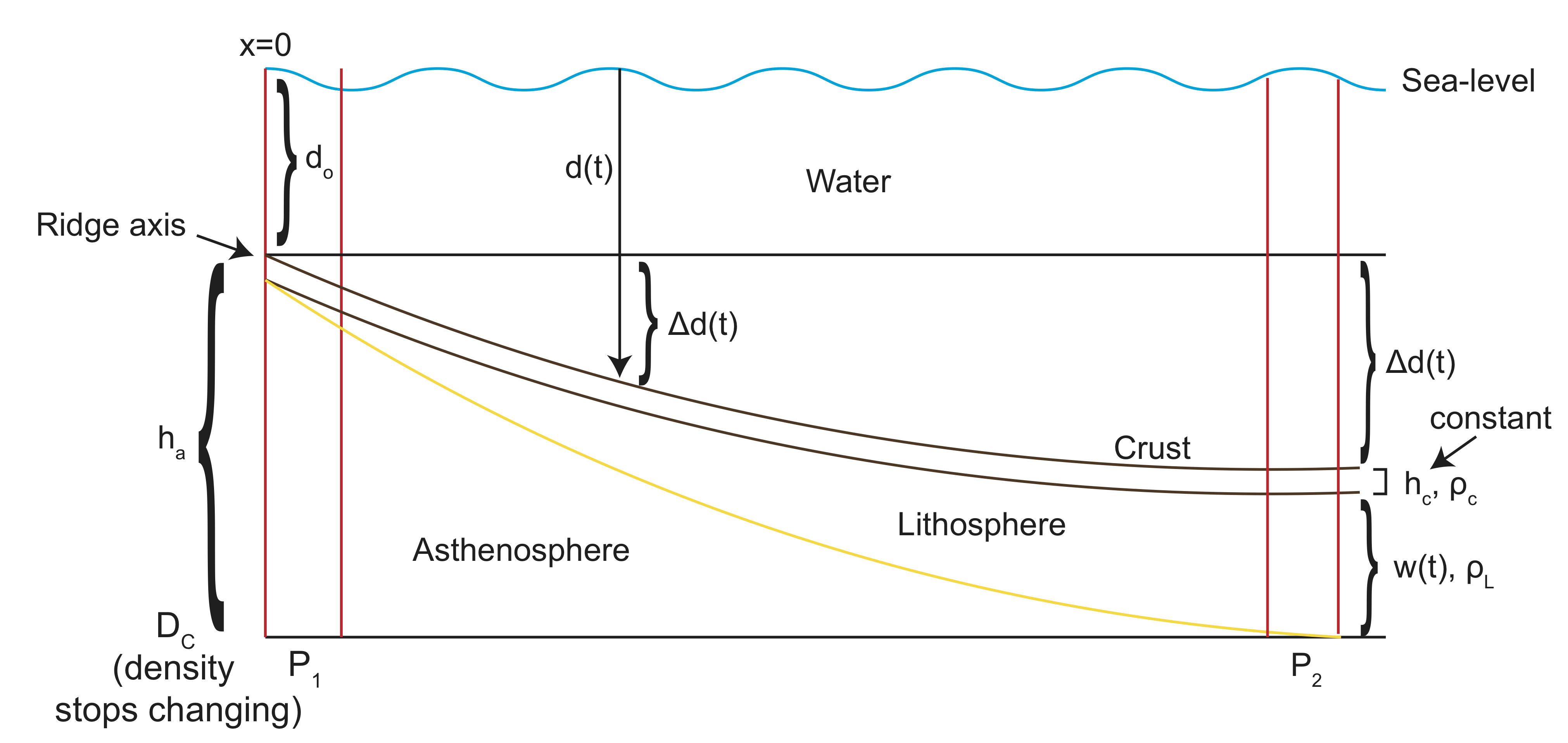
Isostatic balance can be used to determine the amount the ocean depth increases relative to its original depth, \(\Delta d(t)\). The total depth is given by:
\[d(t)=d_o+\Delta d(t) ?\]
We know, from the solving the diffusion equation, that the lithosphere cools and thickens. The thickness of the lithosphere, \(w(t)\), corresponds to following an isotherm (e.g., 1000 C) and assuming that the mass associated with the warmer material is small and can be ignored.
Notice that we can ignore the thickness of water above the ridge, because this water also exists everywhere else. Therefore, when balancing the pressure in two columns, one at the ridge and one some distance away, we only need to consider the layers that exist beneath the ridge height. At the ridge this is \(h_c + h_a\), where \(h_a\) is the asthenosphere. At some distance away (corresponding to time of cooling or plate age of, \(t\)), there are three layers:
- the deepening ocean relative to the ridge given by \(\Delta d(t)\)
- the oceanic crust, \(h_c\)
- the lithosphere thickness (not including the crust), \(w(t)\)
Also note that, \(h_c\) exists in both columns, so \(h_a=\Delta d(t)+w(t)\). To complete the problem, write down the pressure balance equation and solve for \(\Delta d(t)\).


