3.2: Layered Structure of a Planet
- Page ID
- 3520
\( \newcommand{\vecs}[1]{\overset { \scriptstyle \rightharpoonup} {\mathbf{#1}} } \)
\( \newcommand{\vecd}[1]{\overset{-\!-\!\rightharpoonup}{\vphantom{a}\smash {#1}}} \)
\( \newcommand{\id}{\mathrm{id}}\) \( \newcommand{\Span}{\mathrm{span}}\)
( \newcommand{\kernel}{\mathrm{null}\,}\) \( \newcommand{\range}{\mathrm{range}\,}\)
\( \newcommand{\RealPart}{\mathrm{Re}}\) \( \newcommand{\ImaginaryPart}{\mathrm{Im}}\)
\( \newcommand{\Argument}{\mathrm{Arg}}\) \( \newcommand{\norm}[1]{\| #1 \|}\)
\( \newcommand{\inner}[2]{\langle #1, #2 \rangle}\)
\( \newcommand{\Span}{\mathrm{span}}\)
\( \newcommand{\id}{\mathrm{id}}\)
\( \newcommand{\Span}{\mathrm{span}}\)
\( \newcommand{\kernel}{\mathrm{null}\,}\)
\( \newcommand{\range}{\mathrm{range}\,}\)
\( \newcommand{\RealPart}{\mathrm{Re}}\)
\( \newcommand{\ImaginaryPart}{\mathrm{Im}}\)
\( \newcommand{\Argument}{\mathrm{Arg}}\)
\( \newcommand{\norm}[1]{\| #1 \|}\)
\( \newcommand{\inner}[2]{\langle #1, #2 \rangle}\)
\( \newcommand{\Span}{\mathrm{span}}\) \( \newcommand{\AA}{\unicode[.8,0]{x212B}}\)
\( \newcommand{\vectorA}[1]{\vec{#1}} % arrow\)
\( \newcommand{\vectorAt}[1]{\vec{\text{#1}}} % arrow\)
\( \newcommand{\vectorB}[1]{\overset { \scriptstyle \rightharpoonup} {\mathbf{#1}} } \)
\( \newcommand{\vectorC}[1]{\textbf{#1}} \)
\( \newcommand{\vectorD}[1]{\overrightarrow{#1}} \)
\( \newcommand{\vectorDt}[1]{\overrightarrow{\text{#1}}} \)
\( \newcommand{\vectE}[1]{\overset{-\!-\!\rightharpoonup}{\vphantom{a}\smash{\mathbf {#1}}}} \)
\( \newcommand{\vecs}[1]{\overset { \scriptstyle \rightharpoonup} {\mathbf{#1}} } \)
\( \newcommand{\vecd}[1]{\overset{-\!-\!\rightharpoonup}{\vphantom{a}\smash {#1}}} \)
\(\newcommand{\avec}{\mathbf a}\) \(\newcommand{\bvec}{\mathbf b}\) \(\newcommand{\cvec}{\mathbf c}\) \(\newcommand{\dvec}{\mathbf d}\) \(\newcommand{\dtil}{\widetilde{\mathbf d}}\) \(\newcommand{\evec}{\mathbf e}\) \(\newcommand{\fvec}{\mathbf f}\) \(\newcommand{\nvec}{\mathbf n}\) \(\newcommand{\pvec}{\mathbf p}\) \(\newcommand{\qvec}{\mathbf q}\) \(\newcommand{\svec}{\mathbf s}\) \(\newcommand{\tvec}{\mathbf t}\) \(\newcommand{\uvec}{\mathbf u}\) \(\newcommand{\vvec}{\mathbf v}\) \(\newcommand{\wvec}{\mathbf w}\) \(\newcommand{\xvec}{\mathbf x}\) \(\newcommand{\yvec}{\mathbf y}\) \(\newcommand{\zvec}{\mathbf z}\) \(\newcommand{\rvec}{\mathbf r}\) \(\newcommand{\mvec}{\mathbf m}\) \(\newcommand{\zerovec}{\mathbf 0}\) \(\newcommand{\onevec}{\mathbf 1}\) \(\newcommand{\real}{\mathbb R}\) \(\newcommand{\twovec}[2]{\left[\begin{array}{r}#1 \\ #2 \end{array}\right]}\) \(\newcommand{\ctwovec}[2]{\left[\begin{array}{c}#1 \\ #2 \end{array}\right]}\) \(\newcommand{\threevec}[3]{\left[\begin{array}{r}#1 \\ #2 \\ #3 \end{array}\right]}\) \(\newcommand{\cthreevec}[3]{\left[\begin{array}{c}#1 \\ #2 \\ #3 \end{array}\right]}\) \(\newcommand{\fourvec}[4]{\left[\begin{array}{r}#1 \\ #2 \\ #3 \\ #4 \end{array}\right]}\) \(\newcommand{\cfourvec}[4]{\left[\begin{array}{c}#1 \\ #2 \\ #3 \\ #4 \end{array}\right]}\) \(\newcommand{\fivevec}[5]{\left[\begin{array}{r}#1 \\ #2 \\ #3 \\ #4 \\ #5 \\ \end{array}\right]}\) \(\newcommand{\cfivevec}[5]{\left[\begin{array}{c}#1 \\ #2 \\ #3 \\ #4 \\ #5 \\ \end{array}\right]}\) \(\newcommand{\mattwo}[4]{\left[\begin{array}{rr}#1 \amp #2 \\ #3 \amp #4 \\ \end{array}\right]}\) \(\newcommand{\laspan}[1]{\text{Span}\{#1\}}\) \(\newcommand{\bcal}{\cal B}\) \(\newcommand{\ccal}{\cal C}\) \(\newcommand{\scal}{\cal S}\) \(\newcommand{\wcal}{\cal W}\) \(\newcommand{\ecal}{\cal E}\) \(\newcommand{\coords}[2]{\left\{#1\right\}_{#2}}\) \(\newcommand{\gray}[1]{\color{gray}{#1}}\) \(\newcommand{\lgray}[1]{\color{lightgray}{#1}}\) \(\newcommand{\rank}{\operatorname{rank}}\) \(\newcommand{\row}{\text{Row}}\) \(\newcommand{\col}{\text{Col}}\) \(\renewcommand{\row}{\text{Row}}\) \(\newcommand{\nul}{\text{Nul}}\) \(\newcommand{\var}{\text{Var}}\) \(\newcommand{\corr}{\text{corr}}\) \(\newcommand{\len}[1]{\left|#1\right|}\) \(\newcommand{\bbar}{\overline{\bvec}}\) \(\newcommand{\bhat}{\widehat{\bvec}}\) \(\newcommand{\bperp}{\bvec^\perp}\) \(\newcommand{\xhat}{\widehat{\xvec}}\) \(\newcommand{\vhat}{\widehat{\vvec}}\) \(\newcommand{\uhat}{\widehat{\uvec}}\) \(\newcommand{\what}{\widehat{\wvec}}\) \(\newcommand{\Sighat}{\widehat{\Sigma}}\) \(\newcommand{\lt}{<}\) \(\newcommand{\gt}{>}\) \(\newcommand{\amp}{&}\) \(\definecolor{fillinmathshade}{gray}{0.9}\)Once the mass of a planet or moon is known, the next thing a planetary scientist want to know is what is the layered structure inside the planetary object. Does the object have a dense iron core? Or, is the object homogeneous? How thick is observed crustal (or ice) layer that is observed at the surface. This information is more difficult to determine, but with just one more piece of information and some educated assumptions about the plausible composition and density), it is possible to determine the basic layered structure. The additional piece of necessary information is the moment of inertia. Below, we will describe one way that the moment of inertia can be determined by using an orbiter to detect measure the shape of the gravitational field around the planetary object. First, let's review moment of inertia.
Moment of Inertia
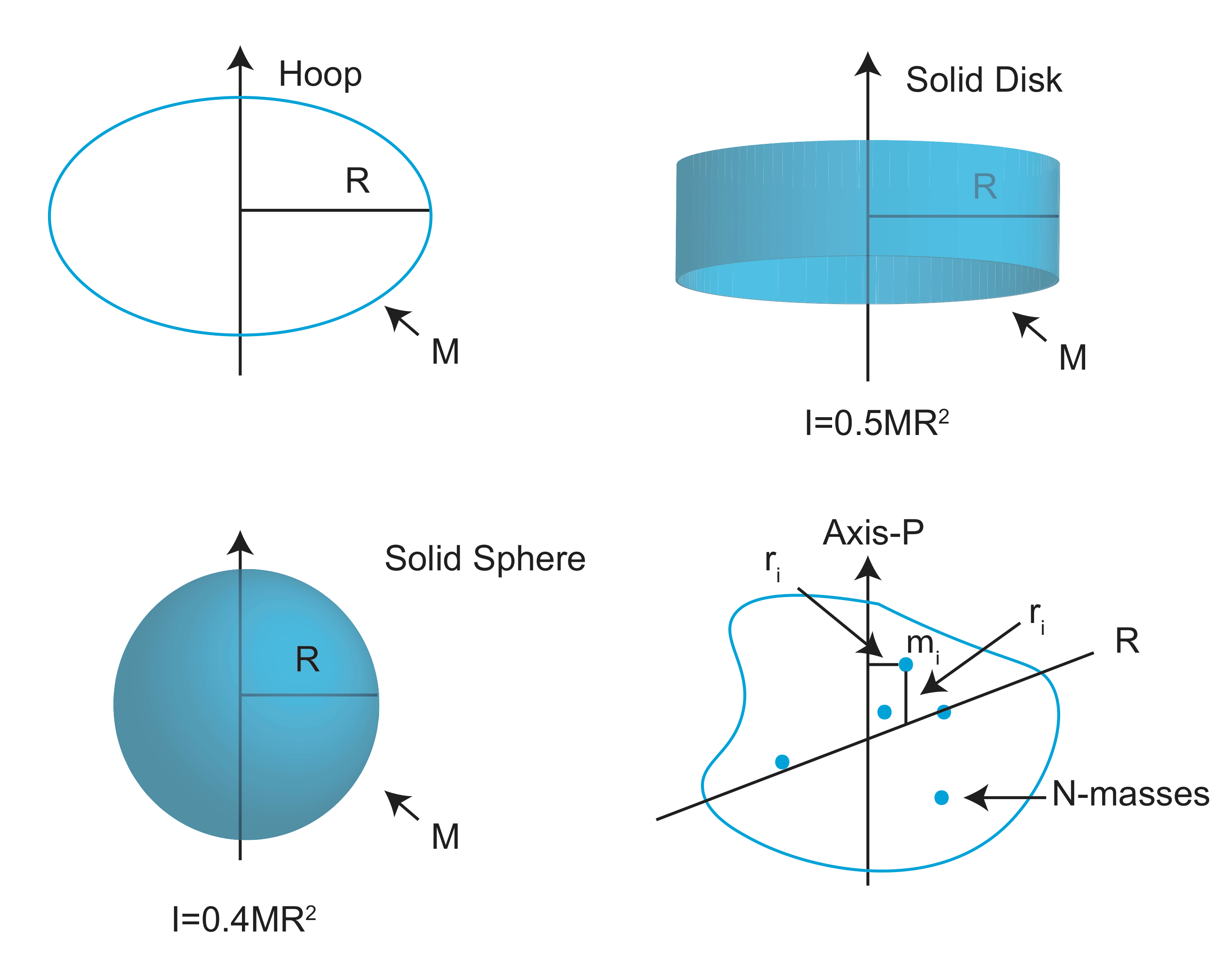
A moment of inertia quantifies the distribution of mass of an object relative to an axis. Consider the irregular shaped object in the figure below, with an axis P. The mass of the object can be considered as many individual point masses, \(m_i\), each located a distance \(r_i\) from the axis. Note this distance, \(r_i\) is measured along a line that is perpendicular to the axis located at the height of the point mass. The moment of inertia of axis P is given as the sum over all the point masses,
\[I_P=\sum_{i=1}^{N} m_i{r_i}^2\]
This sum gives a scalar value. Also, note that if a different axis is used, the moment of inertia will be different.
For most commonly-used shapes this sum can be calculated as an explicit integral and there are analytic expressions that depend on the total mass of the object. For example the moment of inertia of a solid disk about an axis through the center is \(0.5MR^2\), whereas the moment of inertia for a sphere is \(0.4MR^2\). More examples of moment of inertia for different shapes can be found here.

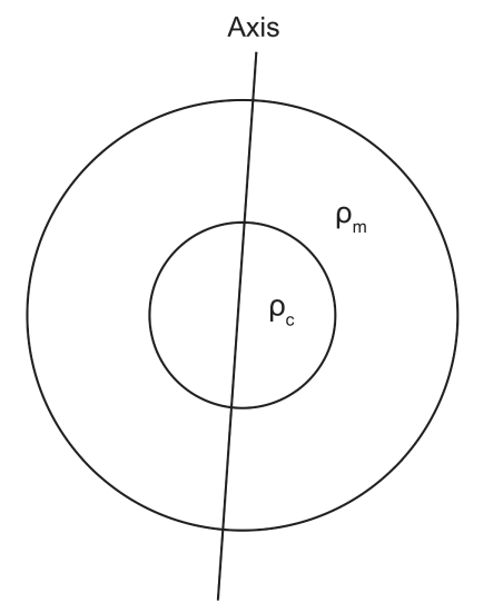
Of particular interest for planetary structure is the how the moment of inertia changes as one goes from a solid sphere with a uniform density to a sphere with higher density material at is core. For a sphere with a higher density core and lower density outer layer, the moment of inertia will decrease relative to the moment of inertia of a homogeneous sphere.

When \(\rho_c>\rho_m\), more mass is closer to the axis compared to a uniform sphere, this means that more mass is at smaller distances from an axis through the center of the sphere, and therefore the sums of \(m_i r_i^2\) will be smaller, so the moment of inertia will be smaller for the layered sphere
\[I_{layered} < 0.4 MR^2 \nonumber\]
Caution: this is for a layered sphere with higher density material at the core relative to the outer layer. If the denser layer was on the outside the moment of inertia would be bigger. However, for planets, the denser material sinks to the core due to gravitational segregation, so the layered structure always has a higher density for the deeper layer.
In addition, its important to notice that the moment of inertia depends on the mass, but also on the radius. Therefore, both a higher density or larger radius of the inner layer could lead a larger moment of inertia, so there are multiple models with the same total mass that could give the same moment of inertia.
Example: Trade-off between density and Radius
The bulk density of the earth is about \(\rho_{bulk}=5550\) kg/m\(^3\) and the average moment of inertia is \(0.33 MR_e^2\).
These two models for the mantle density, \(\rho_m\), the core density \(\rho_c\) and layer thickness both give the same total mass and moment of inertia:
- Model 1: \(\rho_m=4000\) kg/m\(^3\), \(\rho_c=10800\) kg/m\(^3\), with the ratio of radii as \(\frac{r_c}{r_m} =0.6\)
- Model 2: \(\rho_m=2850\) kg/m\(^3\), \(\rho_c=8120\) kg/m\(^3\), with the ratio of radii as \(\frac{r_c}{r_m} =0.8\)
Moment of Inertia of Ellipsoidal Object, like Earth
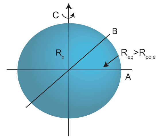
It is important to remember that Earth, and planets in general, are not spheres, they are ellipsoids. This means that there shape is described by two moments of inertia. The moment of inertia around the axis aligned with the spinning axis is usually given then symbol \(C\), while the moment of inertia around an axis through the equator is given the symbol \(A\). The axis through the equator can have any orientation since the equator is an actual circle. (If the shape were also elliptical, then the axis perpendicular to A would be denoted B).

If we knew \(C\) and \(A\), we could use \(m\), \(R\), and \(\rho_{bulk}\) to estimate the internal layered structure of the planet. Even with this information there will be trade-offs between the assumed values of the densities and thickness of the layers. Therefore, other observation of the surface of the planet, including spectral information, can provide constraints on the composition (and density) of the surface layer. For more precise models, other data is needed that constrains the bulk composition of the planet and then petrologic calculations are used to determine the plausible compositions. For the Earth, this extra information comes from the composition of meteorites, which were the building blocks of the planet, as well as xenoliths (mantle rocks brought to the surface through volcanic activity).
Advanced Topic: Determining Moment of Inertia for Planets
If we know the moment of inertia of a planet and its mass, it is possible to determine simple models of the layered density structure of the planet. The layered density structure is defined by the thickness of the layers and the density of each layer. Usually, it is possible to determine reasonable two-layered structures (i.e., radius of the core and thickness of the mantle) if we have additional information about the composition and/or density at the surface of the planet.
Procedure for Determining Moment of Inertia
The main assumption in the following procedure is that the planet behaves like a fluid (flows viscously) over long periods of time (e.g., a million years). This is called the hydrostatic assumption. This is a reasonable assumption for rocky planets, which have mantle compositions similar to the Earth.
- The shape of spinning planets is that of an oblate spheroid that is slightly broader at the equator and shorter at the poles. The oblate shape is quantified by the the flattening, \(f\). The flattening of a rotating, fluid planet, with a polar radius, \(c\), and equatorial radius, \(a\), is given by:
\[f=\frac{a-c}{a}\]
The equatorial radius is larger because the spinning motion of the planet (centripetal force) causes mass to move to the equator and away from the poles. While this is a simple equation, it is actually not easy to get accurate measurements of the equatorial and polar radii of a planetary object. However, the flattening can be determined by measuring the gravitational potential field, which will mimic the oblate shape of the planet, through the orbit of satellites or an orbiter. The orbit will be perturbed by the non-spherical potential field, and these perturbations can be related to the actual shape of the gravitational potential.
The shape of the gravitational potential field is usually expressed in terms of functions called spherical harmonics. Think of these as sines and cosines, but instead of depending on just one angle, they depend on both longitude and latitude. It is possible to use an infinite sum of sines and cosines, of varying frequency and amplitude, to represent any other function that depends on just one variable. Likewise, it is possible to represent any 3D field in spherical coordinates using an infinite sum of spherical harmonics. It turns out that if you do this, the amplitude of the third term in the sum is directly related to the flattened (oblate) shape of an object. This term, called the ellipticity coefficient, is usually given the symbol, \(J_2\), and depends on two of the moments of inertia of the object,
\[ J_2 = \frac{C-A}{Ma^2}\]
Therefore, by measuring the orbits of satellite, we can get a first-order estimate of the flattening by just keeping two terms from the spherical harmonic representation of the gravity field,
\[f_{hyd}\approx\frac{3}{2}J_2+\frac{1}{2}\frac{a^3\omega^2}{2GM} \label{fhyd}\]
However, remember that we are trying to determine the internal layering structure of a planet, so we are interested in the moment of inertia \(\frac{C}{Ma^2}\), but the ellipticity depends on two moments, \(C\) and \(A\). Therefore, planetary scientists came up with another, approximate, way to express the flattening that only depends on \(\frac{C}{Ma^2}\). You know it is not easy to come up with the approximation by the fact that this equation has a name, the Darwin-Radau Approximation (not the Darwin of survival of the fittest).
- The Darwin-Radau Approximation provides a second approximate expression for the hydrostatic flattening,
\[f_{hyd} \approx \frac{\frac{5}{2}\frac{a^3\omega^2}{GM}}{1+\frac{25}{4}\left(1-\frac{3}{2}\frac{C}{Ma^2}\right)^2}\]
In this equation, everything can be measured/observed, including \(f_{hyd}\) from equation \ref{fhyd}, which means that the equation can be used to solve for the moment of inertia factor \(\frac{C}{Ma^2}\),
\[\frac{C}{Ma^2} \approx \frac{2}{3}\left(1-\sqrt{\frac{2}{5}\frac{\frac{a^3\omega^2}{GM}}{f_{hyd}}-\frac{4}{25}}\right)\]
Using this equation, with observations of the planetary mass, the equatorial radius and \(f_{hyd}\) from the gravitational potential field, the moment of inertia factor of the planet can be determined. With this information, simple models of the the two layered structure can be made that also match the total mass of the planet. It is usually necessary to also have some educated guesses as to the expected average density of the mantle and the core.


