
1.5: Viscous Deformation
- Page ID
- 3535

\( \newcommand{\vecs}[1]{\overset { \scriptstyle \rightharpoonup} {\mathbf{#1}} } \)
\( \newcommand{\vecd}[1]{\overset{-\!-\!\rightharpoonup}{\vphantom{a}\smash {#1}}} \)
\( \newcommand{\id}{\mathrm{id}}\) \( \newcommand{\Span}{\mathrm{span}}\)
( \newcommand{\kernel}{\mathrm{null}\,}\) \( \newcommand{\range}{\mathrm{range}\,}\)
\( \newcommand{\RealPart}{\mathrm{Re}}\) \( \newcommand{\ImaginaryPart}{\mathrm{Im}}\)
\( \newcommand{\Argument}{\mathrm{Arg}}\) \( \newcommand{\norm}[1]{\| #1 \|}\)
\( \newcommand{\inner}[2]{\langle #1, #2 \rangle}\)
\( \newcommand{\Span}{\mathrm{span}}\)
\( \newcommand{\id}{\mathrm{id}}\)
\( \newcommand{\Span}{\mathrm{span}}\)
\( \newcommand{\kernel}{\mathrm{null}\,}\)
\( \newcommand{\range}{\mathrm{range}\,}\)
\( \newcommand{\RealPart}{\mathrm{Re}}\)
\( \newcommand{\ImaginaryPart}{\mathrm{Im}}\)
\( \newcommand{\Argument}{\mathrm{Arg}}\)
\( \newcommand{\norm}[1]{\| #1 \|}\)
\( \newcommand{\inner}[2]{\langle #1, #2 \rangle}\)
\( \newcommand{\Span}{\mathrm{span}}\) \( \newcommand{\AA}{\unicode[.8,0]{x212B}}\)
\( \newcommand{\vectorA}[1]{\vec{#1}} % arrow\)
\( \newcommand{\vectorAt}[1]{\vec{\text{#1}}} % arrow\)
\( \newcommand{\vectorB}[1]{\overset { \scriptstyle \rightharpoonup} {\mathbf{#1}} } \)
\( \newcommand{\vectorC}[1]{\textbf{#1}} \)
\( \newcommand{\vectorD}[1]{\overrightarrow{#1}} \)
\( \newcommand{\vectorDt}[1]{\overrightarrow{\text{#1}}} \)
\( \newcommand{\vectE}[1]{\overset{-\!-\!\rightharpoonup}{\vphantom{a}\smash{\mathbf {#1}}}} \)
\( \newcommand{\vecs}[1]{\overset { \scriptstyle \rightharpoonup} {\mathbf{#1}} } \)
\( \newcommand{\vecd}[1]{\overset{-\!-\!\rightharpoonup}{\vphantom{a}\smash {#1}}} \)
\(\newcommand{\avec}{\mathbf a}\) \(\newcommand{\bvec}{\mathbf b}\) \(\newcommand{\cvec}{\mathbf c}\) \(\newcommand{\dvec}{\mathbf d}\) \(\newcommand{\dtil}{\widetilde{\mathbf d}}\) \(\newcommand{\evec}{\mathbf e}\) \(\newcommand{\fvec}{\mathbf f}\) \(\newcommand{\nvec}{\mathbf n}\) \(\newcommand{\pvec}{\mathbf p}\) \(\newcommand{\qvec}{\mathbf q}\) \(\newcommand{\svec}{\mathbf s}\) \(\newcommand{\tvec}{\mathbf t}\) \(\newcommand{\uvec}{\mathbf u}\) \(\newcommand{\vvec}{\mathbf v}\) \(\newcommand{\wvec}{\mathbf w}\) \(\newcommand{\xvec}{\mathbf x}\) \(\newcommand{\yvec}{\mathbf y}\) \(\newcommand{\zvec}{\mathbf z}\) \(\newcommand{\rvec}{\mathbf r}\) \(\newcommand{\mvec}{\mathbf m}\) \(\newcommand{\zerovec}{\mathbf 0}\) \(\newcommand{\onevec}{\mathbf 1}\) \(\newcommand{\real}{\mathbb R}\) \(\newcommand{\twovec}[2]{\left[\begin{array}{r}#1 \\ #2 \end{array}\right]}\) \(\newcommand{\ctwovec}[2]{\left[\begin{array}{c}#1 \\ #2 \end{array}\right]}\) \(\newcommand{\threevec}[3]{\left[\begin{array}{r}#1 \\ #2 \\ #3 \end{array}\right]}\) \(\newcommand{\cthreevec}[3]{\left[\begin{array}{c}#1 \\ #2 \\ #3 \end{array}\right]}\) \(\newcommand{\fourvec}[4]{\left[\begin{array}{r}#1 \\ #2 \\ #3 \\ #4 \end{array}\right]}\) \(\newcommand{\cfourvec}[4]{\left[\begin{array}{c}#1 \\ #2 \\ #3 \\ #4 \end{array}\right]}\) \(\newcommand{\fivevec}[5]{\left[\begin{array}{r}#1 \\ #2 \\ #3 \\ #4 \\ #5 \\ \end{array}\right]}\) \(\newcommand{\cfivevec}[5]{\left[\begin{array}{c}#1 \\ #2 \\ #3 \\ #4 \\ #5 \\ \end{array}\right]}\) \(\newcommand{\mattwo}[4]{\left[\begin{array}{rr}#1 \amp #2 \\ #3 \amp #4 \\ \end{array}\right]}\) \(\newcommand{\laspan}[1]{\text{Span}\{#1\}}\) \(\newcommand{\bcal}{\cal B}\) \(\newcommand{\ccal}{\cal C}\) \(\newcommand{\scal}{\cal S}\) \(\newcommand{\wcal}{\cal W}\) \(\newcommand{\ecal}{\cal E}\) \(\newcommand{\coords}[2]{\left\{#1\right\}_{#2}}\) \(\newcommand{\gray}[1]{\color{gray}{#1}}\) \(\newcommand{\lgray}[1]{\color{lightgray}{#1}}\) \(\newcommand{\rank}{\operatorname{rank}}\) \(\newcommand{\row}{\text{Row}}\) \(\newcommand{\col}{\text{Col}}\) \(\renewcommand{\row}{\text{Row}}\) \(\newcommand{\nul}{\text{Nul}}\) \(\newcommand{\var}{\text{Var}}\) \(\newcommand{\corr}{\text{corr}}\) \(\newcommand{\len}[1]{\left|#1\right|}\) \(\newcommand{\bbar}{\overline{\bvec}}\) \(\newcommand{\bhat}{\widehat{\bvec}}\) \(\newcommand{\bperp}{\bvec^\perp}\) \(\newcommand{\xhat}{\widehat{\xvec}}\) \(\newcommand{\vhat}{\widehat{\vvec}}\) \(\newcommand{\uhat}{\widehat{\uvec}}\) \(\newcommand{\what}{\widehat{\wvec}}\) \(\newcommand{\Sighat}{\widehat{\Sigma}}\) \(\newcommand{\lt}{<}\) \(\newcommand{\gt}{>}\) \(\newcommand{\amp}{&}\) \(\definecolor{fillinmathshade}{gray}{0.9}\)The flow of liquids, like water, honey, oil, and magma, is described as viscous flow or viscous deformation. Similar to elastic deformation we can ask how the deformation is related to the stress during viscous deformation. In this case, the stress is related to the strain-rate \(\dot{\epsilon} = \frac{d\epsilon}{dt}\), rather than the strain \(\epsilon\) through the viscosity \(\eta\), (the greek symbol eta):
\[ \sigma = 2 \eta \dot{\epsilon} \]
This equation states that the stress in a viscous material is proportional to how fast it is deforming (the strain-rate). The factor of 2 is there for mathematical convenience in full 3-D descriptions of viscous deformation. The stress has units of Pascals and the strain-rate has units of 1/s, so the viscosity has units of Pa*s. The viscosity can be thought of as the resistance to flow. Higher viscosity indicates more resistance to flow. This can be seen more readily, by rewriting the equation above as:
\[\dot{\epsilon} = \frac{\sigma}{2\eta} \]
For a given applied stress \(\sigma\) a higher viscosity will result in a lower strain-rate \(\dot{\epsilon}\). Viscosity is typically dependent on temperature and composition. The viscosity of some familiar liquids are given in Table 1.5.1. Notice that the viscosity ranges over five orders of magnitude (0.001 to 100 Pa s) for these familiar liquids. For example the difference in viscosity of water and oil is a factor of 10, whereas the difference in viscosity between water and honey is 10,000. Materials with lower viscosity deform (flow) faster than materials with a higher viscosity.
| Material | Viscosity (at 20 C) (Pa s) |
|---|---|
| water | 0.0010 |
| milk | 0.0020 |
| olive oil | 0.010 |
| honey | 10.0 |
| toothpaste | 70.0 |
| tar | 100.00 |
Viscous Deformation in Solid Rocks or Ice
While we normally think of rocks as being hard, elastic materials that break, the rheology of rocks (and ice) is in fact both elastic and viscous, but these two different responses occur at different time-scales. The short-term deformation of rocks is best described as elastic with brittle failure and applies to processes like earthquakes (timescale of 1-1000 years between events) and propagation of seismic waves (timescale < seconds). This short term response dominates at cold temperatures and low pressures typically found in the crust. However, even at the high pressures and temperatures of the deep mantle the elastic behavior of the rock allows for the transmission of seismic waves due to the very short timescale of this process. The long term deformation of the lithosphere and the mantle is best described as viscous flow. At the higher pressures and temperatures of the deep lithosphere and mantle, deformation of grains by viscous mechanisms occurs more readily than elastic or brittle deformation. However, it is a very slow process with mantle flow occurring at velocities of 1 to 20 cm/yr, at time-scales of a miliion years or more. Viscosity in the mantle is strongly dependent on temperature, as well as stress and rock composition. Typical values of viscosity in the mantle are \(10^{18}\) to \(10^{24}\) Pa s. These are large numbers, but similar to the more common materials discussed above, the variation of rock viscosity in the mantle is about 6 orders of magnitude. Ice is also a viscous and elastic material. The viscous behavior of ice can be see in ice streams that flow downhill carry ice away from large glaciers. The viscosity of ice is typically in the range around \(10^{13}\) at \(0^\circ C\) to \(10^{14}\) at \(-10^\circ C\) Pa s.
The viscous deformation of the rock (and ice) occurs by crystal-scale deformation (called creep). In this solid-state creep the grains themselves deform as individual atoms (a lot of them) or planes of atoms (called dislocations) move within the grains. These processes of solid state creep are ultimately controlled by how slowly atoms move through the crystal (a diffusive process), which is why the time-scale is so long and the viscosity is so high. Its important to remember that at high pressure, the rocks are flowing but they are still solid. High temperatures (around 1200-1400 C) and relatively lower pressure are needed to cause the rock to melt and form magma.
Applications of Viscous Flow in/on the Earth
In this section we will use viscous flow to consider the deformation of solid rock and ice behaving as a viscous fluid (termed solid-state creep) and magma behaving as a viscous fluid. We will consider viscous flow in three settings.
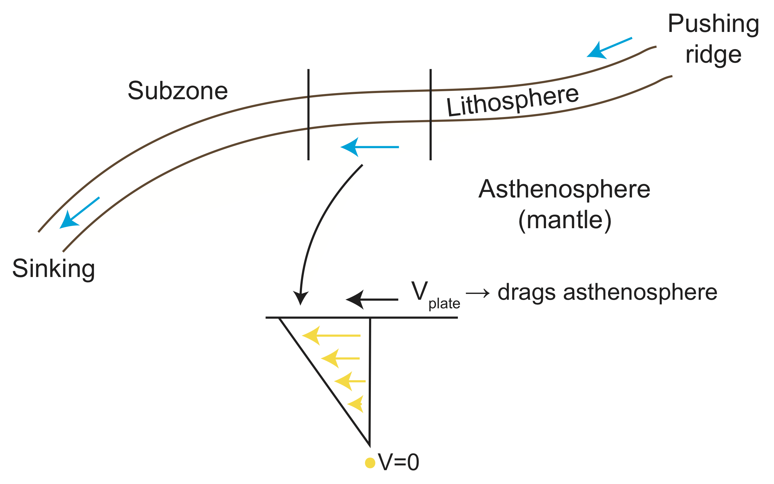
Viscous Drag on a Tectonic Plate
First, we will consider the viscous flow that occurs in the mantle beneath a moving plate (called the asthenosphere). In this case, the tectonics plate (lithosphere) is being moved by two forces. The first force is the slab-pull force caused by sinking tectonic plate (also called a slab) in a subduction zone. The second force moving the plate is the ridge-push force caused by the positive buoyancy of less dense material under a mid-ocean spreading ridge. Figure \(\PageIndex{2}\) shows a profile sketch of a tectonic plate with these forces acting to move the plate across the underlying mantle. The moving plate drags the viscous asthenosphere, and the resistance to this motion is an important force acting on the tectonic plate.
Flow Magma Down a Volcano
When a volcano erupts, magma flows from the vent at the top of the volcano down the sides of the volcano. As the magma cools faster at it edges than in its interior, the flowing magma tends to form its own flow channel: cooled magma forms rock levees on the side of the channel. When the eruption rate of magma is high these channels of of magma can carry liquid magma tens of miles from the vent before the magma cools sufficiently to solidify. We will examine the flow-rate of magma in a simplified magma channel in which we ignore how the magma drags against the sides of the channel and just focus on how the middle of a broad magma channel flows. The flow rate will depend on the viscosity of the magma, but the viscosity of the magma depends on its temperature. As the magma cools, it crystallizes and the network of crystals in the magma strongly increase the viscosity of the magma causing to flow slower.
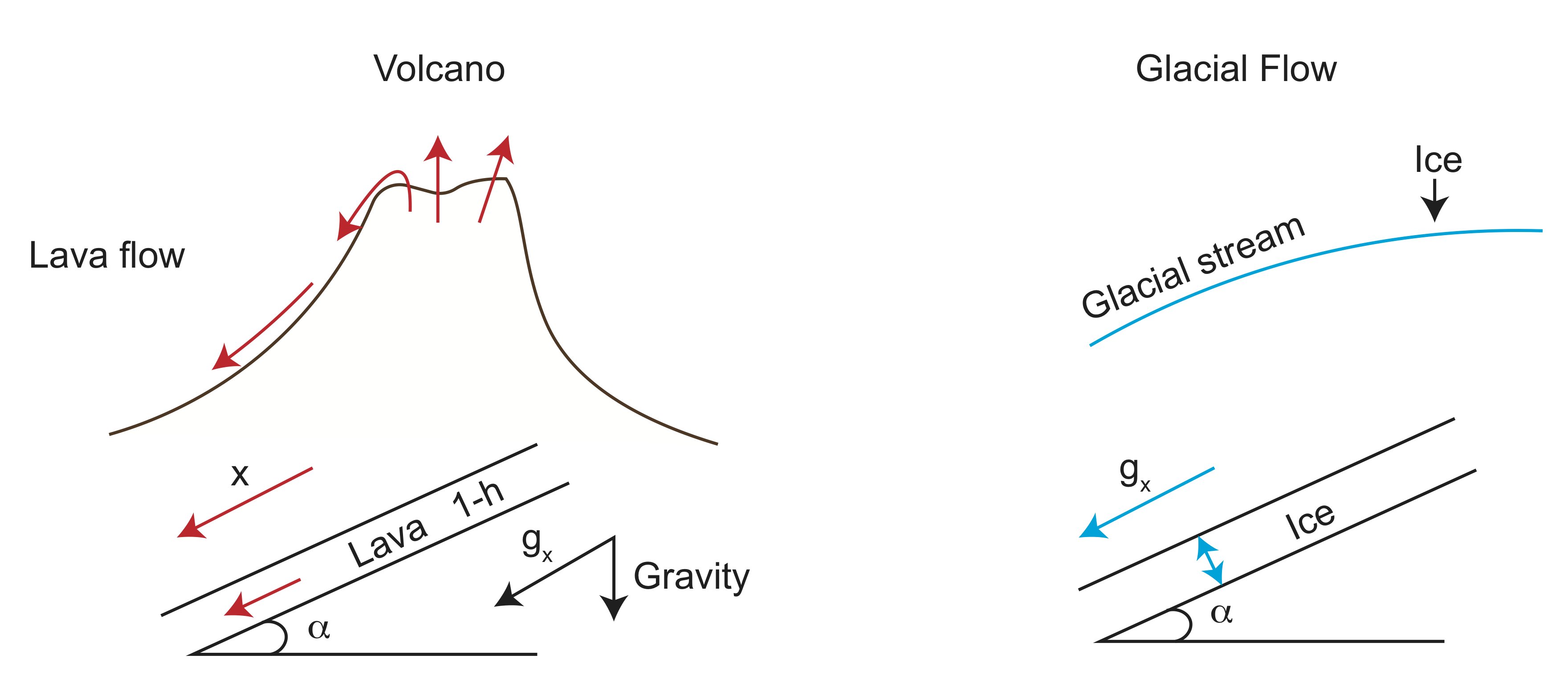
Flow of a Glacial Ice Stream
A glacial ice stream is a region of flowing ice that drains ice away form large glaciers in places like Greenland and Antarctica. These rivers of ice move at rates of about 1 to 100 meters per year, depending on the viscosity (temperature) of the ice, as well as the slope of the land glacial ice stream is flow down. Similar to the case of flowing magma, we can gain some intuition about how this flow by simplifying the geometry and considering only the flow at the center of the ice stream, and the effects of resistance at the base of the flowing ice.
ADD SKETCH (MOVED FROM ABOVE AND ADD TOPOGRAPHY) AND PICTURE OF AN ICE STREAM (FROM WIKIPEDIA).
Flow Through a Pipe
To gain a more intuitive understanding of the parameters and conditions that affect viscous flow, let's begin with a simple model of viscous flow through pipe, like a water pipe in your house or a hose in your backyard.
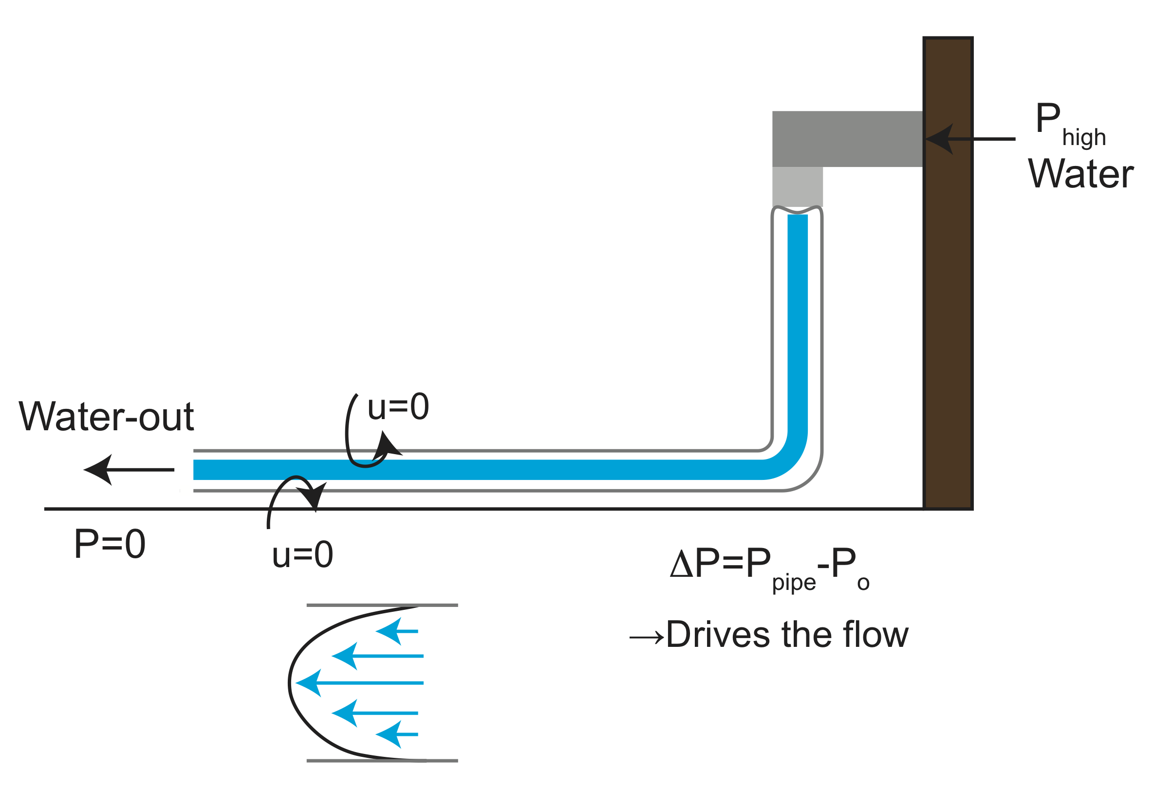
Water flow through the pipe in response to a pressure gradient along the pipe. The pressure at the open end of the pipe \(P_{o}\)=0, while the water is being pushed through the pipe by higher pressure coming from the water being pumped into the street pipes by the utility company. The pressure gradient is given by
\[\Delta P=P_{pipe}-P_{o}\]
Fluid always flows from high pressure to low pressure. It is the pressure difference along the pipe that drives the flow.
Now let's consider for a moment what the fluid flow looks like inside the pipe. Note that at the boundary of the pipe, the pipe is not moving, this means that the fluid directly adjacent to the pipe must also have a velocity of zero. However, a tiny distance away from the wall, the fluid is moving. This creates a gradient in the fluid velocity. The magnitude of the fluid velocity in the x direction, \(u_x\), changes in the y direction, so the gradient of the velocity is non-zero
\[\frac{d u_x}{d y} \neq 0\]
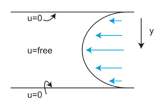
Figure \(\PageIndex{5}\): Inside a pipe the fluid that touches the pipe wall is not moving (u=0). The velocity at the center of the pipe is driven by the pressure gradient in the pipe. Therefore, there is a gradient in the velocity in the pipe.
Let's pause for a moment to consider the units associated with this equation. Velocity has units of meters/second (m/s) while length has units of meters (m)
\[\frac{\frac{m}{s}}{m} = \frac{1}{s} \]
This has units of strain-rate (1/s)
\[\dot{\epsilon}=\frac{1}{2} \frac{d u_x}{d y}\]
Recall that strain is given by the gradient in displacement
\[\epsilon = \frac{\Delta x}{y}\]
Likewise, velocity is the rate of displacement, therefore the gradient in the rate of displacement results in a strain rate.
Estimating Strain Rate
It is useful to pause now to get an order of magnitude estimate of strain-rate. To do this, let's look at the plot below comparing strain as a function of time.
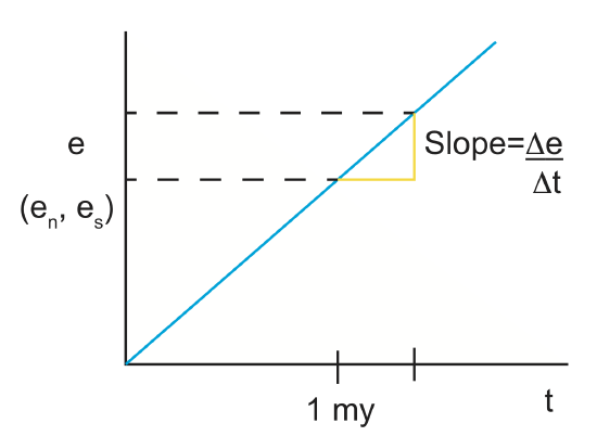
The slope is \(\frac{\Delta e}{\Delta t}\)
Let's assume we have a strain of 0.3 that has accrued over a time period of 1 my:
\[\begin{align*}&=\dfrac{0.3}{1my}\cdot \frac{-1 my}{1\times10^6 yr} \cdot \frac{1 yr}{3.15\times10^7 s} \\[4pt] &= \frac{0.1}{1\times10^{13}}=1\times10^{-14} s^{-1} \end{align*}\]
Strain-rates along plate boundaries and near subducting plates are typically about \(1\times10^{-15}\) to \(1\times10^{-12} s^{-1}\). The rates depend both on the magnitude of the stresses and the magnitude of the viscosity, which is strongly temperature dependent. The viscosity of the asthenosphere is about \(1\times10^{18}\) to \(1\times10^{21}\) Pa-s (Pascal seconds), while viscosity inside a sinking tectonic plate may be as high as \(1\times10^{25}\) Pa-s. Strain rates are very slow in the solid earth because the viscosity is large. But, other materials can deform much faster, such as an ice flow which deforms at about 1 inch a year. Flowing magma moves even faster, at about 1 inch per minute. Viscosity values for ice range from \(10^{11}-10^{13}\) (Pa)(s) and for lava \(10^{2}-10^{6}\) (Pa)(s).
We often only think about viscous flow in terms of order of magnitude due to the large range in viscosity values. Viscosity depends on a lot of properties of the rock and the physical conditions. Such properties include: composition, grain-size, water in minerals, presence of melt and crystal grains in the melt.
Comparing Elastic and Viscous Deformation
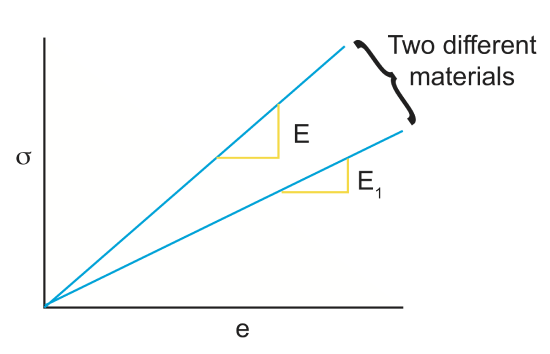
Viscous deformation is different than elastic deformation, in several ways, but one of the primary differences is that for elastic deformation the strain is linear proportional to the stress (\(\sigma = E \epsilon\)), while for viscous deformation it is the strain-rate that is proportional to stress (\(\sigma = \eta \dot{\epsilon}\)). To better understand what this difference means, let's first revisit elastic deformation.
The figure below shows the stress resulting from an applied strain in an elastic material. Different material will have different values for the Young's modulus and thus the same amount of strain will result in different amounts of stress in the material.
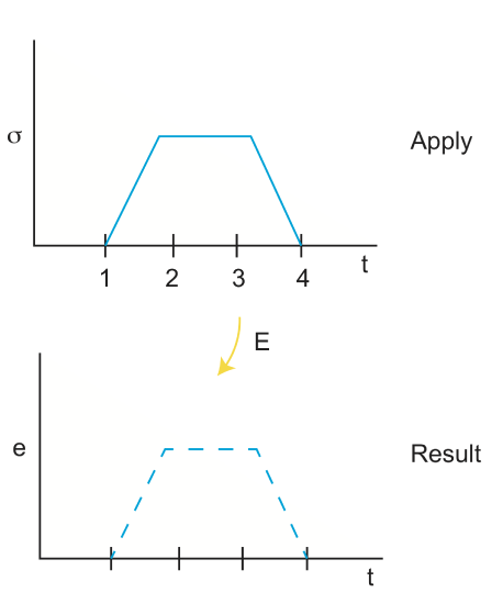
The next figure shows how the strain in a rock deforming elastically is not permanent, but rather it is recoverable. The stress applied to the rock is ramped up from time 1 to time 2 and then held constant from time 2 to time 3. Then the stress is released from time 3 to time 4. The figure below illustrates that the strain in the rock is proportional to the stress and that once the stress returns to zero, the strain also returns to zero.
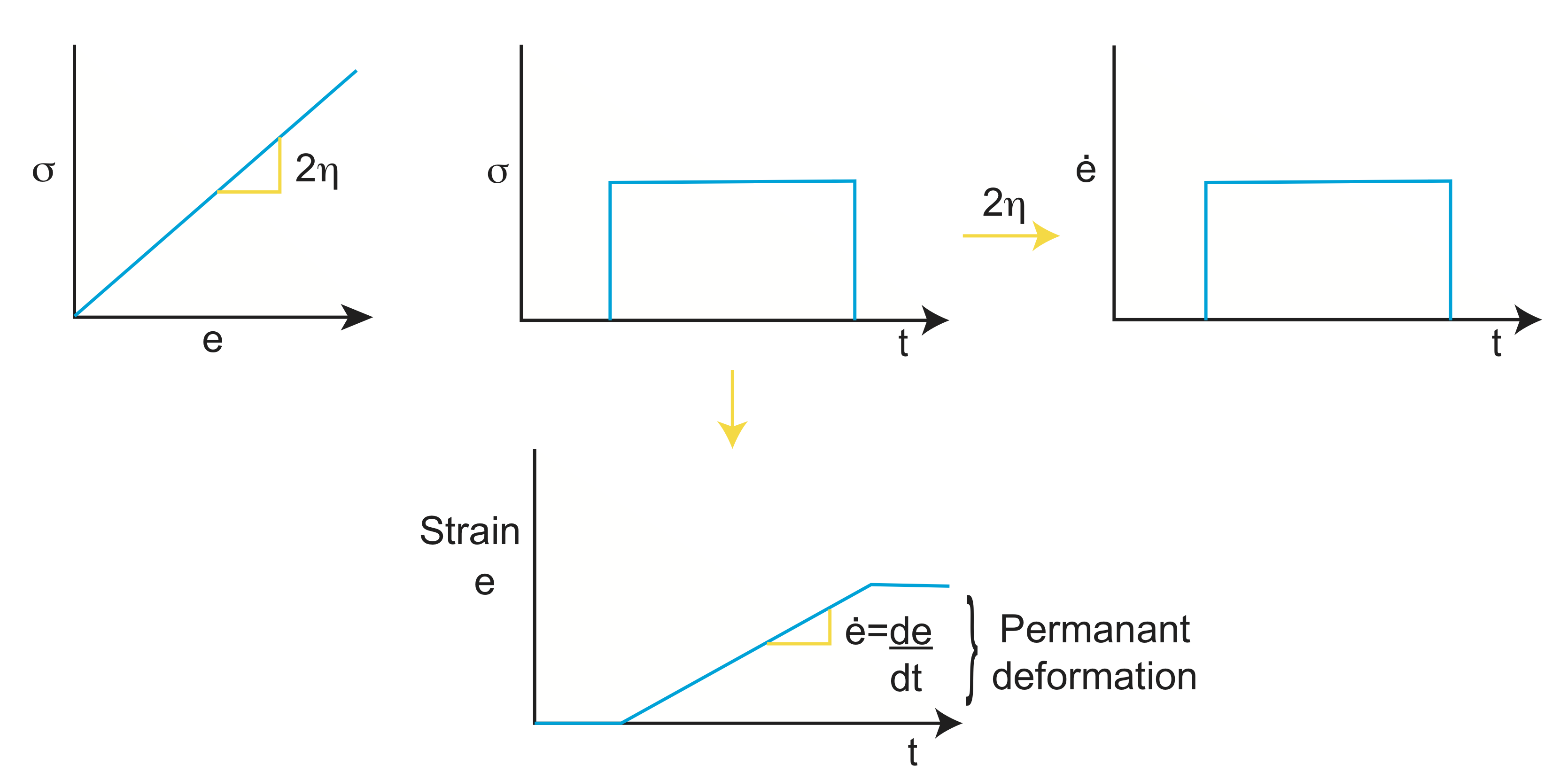
Returning to viscous deformation, we know that viscosity and stress have a time dependent relationship:
\[ \sigma=2\eta\frac{de}{dt}\]
When pulling a stick out of a very viscous fluid like honey or tar, the slower you pull the less stress is required, and the faster you pull, the more stress is needed. For a viscous material, consider that the stress is increased instantaneously, the response of the fluid is to start to flow at a proportional strain-rate. As time goes on the amount of strain in the fluid increases linearly. However, when the stress is returned to zero and the fluid stops moving(the strain-rate is zero), therefore the fluid can not flow back to its original position and instead there is permanent (no-recoverable) deformation. The fact the flow is not recovered does not mean it is not reversible. If the stress is reversed exactly the fluid can be returned to its original position.
Derivation of Viscous flow Equations
The basic equation describing viscous flow \(\sigma = \eta \dot{\epsilon}\) is found by considering conservation of momentum in a fluid. Conservation of momentum is similar to considering a force balance on an element of fluid. Consider an infinitesimal 3D volume of fluid with sides, \(\delta_{x}\), \(\delta_{y}\), \(\delta_{z}\). On each side of the box in the x direction there is a traction acting on the fluid.
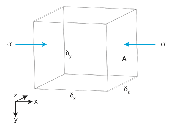
From the figure, we can see that A=\(\delta_{z} \cdot \delta_{y}\). Therefore, the force acting on each side is F=\(\sigma A\).
\[F=\sigma \delta_{z} \delta_{y}\]
Dividing by \(\delta_z\) we get the force per unit length in the z direction.
\[\frac{F}{\delta_z} =\sigma \delta_{y}\]
Using the force per unit length allows us to consider just a 2D cross section of the flow.
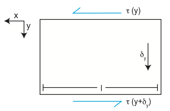
Next, let's consider all the forces acting on the sides of the element of fluid (in 2D). First, on the top and bottom of the fluid element there are shear stress acting tangential to the top and bottom surface. These shear stresses exist in the fluid because the fluid is being held back at the walls of the pipe, while it is free to move in the interior of the pipe.
Finally, we need to balance all the forces acting on the fluid element due to both the normal stresses acting on the sides of the box and the shear stresses acting on the top and bottom of the box. All the forces are directed in the x direction, so the forces should balance (sum to zero).
The normal stresses on the sides are the pressure in the fluid. Recall that there is a pressure gradient along the pipe in the x direction due to the pressure gradient. Therefore the pressure on the upstream side, \(P_1\) is larger than the pressure on the downstream side, \(P_o\). The force (per unit length) on these sides is by the pressure (stress) times the length \(\delta_y\). Similarly the force of the top and bottom are given by the sheear stress times the length, \(\delta_x\). The sum of the forces on all four sides is the
\[P_1 \delta_y - P_o \delta_y + \tau(y) \delta_x - \tau(y+\delta_y) \delta_x = 0 \]
Combining terms we get
\[(P_1 - P_o) \delta_y - (\tau(y+\delta_y) - \tau(y)) \delta_x = 0 \]
Next divide through by both \(\delta_x\) and \(\delta_y\)
\[ \frac{P_1-P_o}{\delta_x} - \frac{\tau(y+\delta_y) - \tau(y)}{\delta_y} = 0 \]
Note the first term is the pressure gradient in the pipe in the x direction, and the second term is the gradient in the shear stress across the pipe
\[ \frac{dP}{dx} = \frac{d\tau}{dy} \]
This equation, describes how the pressure gradient drives the fluid flow, which is resisted by shear stress in the fluid. This general relationship is true regardless of the geometry or boundary conditions on the fluid, and it is a useful concept to use in thinking about how a fluid will deform.
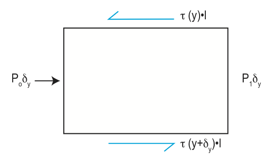
Figure \(\PageIndex{7}\): Conservation of Momentum (MIB: change l to \delta_x)
Finally let's relate shear stress to strain-rate in order to determine the exact form of the fluid flow (velocity) in the pipe. Recall from above that
\[\tau = 2 \eta \dot{\epsilon} = \eta \frac{du}{dy}\]
Substituting in for the shear stress
\[\eta \frac{d^2 u}{dy^2}=\frac{dp}{dx}\]
This is a differential equation, which says that the curvature of the velocity of the fluid in the y direction is equal to the pressure gradient in the x-direction. To determine the shape of the velocity profile, we need to integrate (twice) with respect to y.
\[ u(y)=\frac{1}{2\eta} \frac{dp}{dx} y^2 +c_1 y+c_2 \]
Although we derived this thinking about flow in a pipe, it is the general solution to flow in one direction driven by a pressure gradient. You can see that there are two unknowns in the equation, \(c_o\) and \(c_1\), which are the result of integrating twice to get the velocity. To solve for these constants, we must use information we have about how the flow behaves at the boundaries (this information is referred to as the boundary conditions). Different boundary conditions will lead to different shapes for the velocity profiles. Below we discuss two possible solutions referred to as Couette Flow and flow down an inclined plane.
Couette Flow
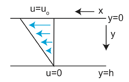
Couette flow is defined by a flow in which there is no applied pressure gradient, but one of the boundaries is moving at a fixed velocity.
\(\frac{dp}{dx}=0 \) and \(u_o \neq 0\)
Therefore, in addition to knowing that the term \(\frac{dp}{dx} =0\) we know the velocity at both the top and bottom boundaries:
u(y=h)=0
u(y=0)=\(u_o\)
By examining the equation for the u(y) and letting \(y=0\) we see that the constant (\(c_2 = u_o\))
Similarly, if we plug in \(u = 0\) and \(y = h\) we find that
\[ u=u_o (1-\frac{y}{h}) \nonumber\]
This equation gives the shape of the velocity profile, between stationary and moving boundaries, and that profile is linear, as shown in the figure above.
Next, we can find the strain rate in the fluid
\[\dot{\epsilon}=\frac{1}{2} \frac{du}{dy} =-\frac{u_o}{2h} \nonumber\]
and the shear stress
\[\sigma=2\eta\dot{\epsilon} = \eta \frac{du}{dy} = -\frac{\eta u_o}{h} \nonumber\]
The negative sign indicates that the shear strain is directed against the direction of flow, in the -x direction.
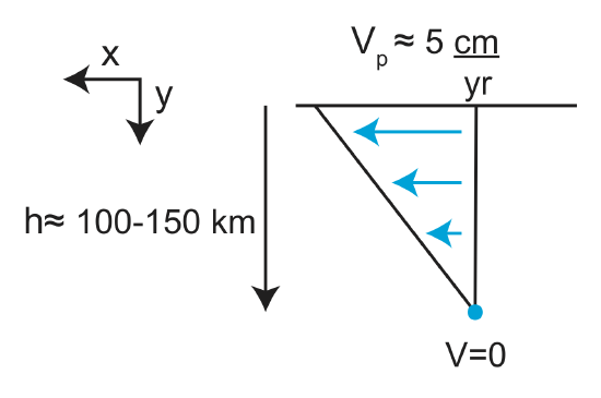
Couette flow can be used to approximate the flow in the mantle be dragged by a moving tectonic plate at the surface above. From the figure below, we estimate that the thickness of the shearing layer beneath the plate \( h = \approx 100-150\) km and the tectonic plate is moving with a velocity of \(v_p \approx 5 \frac{cm}{yr}\). The solution for the Couette flow can then be used to estimate the strain-rate and the shear stress in the asthenosphere below the plate.
Flow Down An Inclined Plane
Now let's consider another geologic application fluid flow down an inclined plane. This geometry can be used to examine flow in a glacial ice stream and flow of magma within channels on the slopes of a volcano.
In this case we consider a layer of flowing fluid with thickness, h, flowing down plane inclined at an angle \(\alpha\). To help solve the problem using the equations we already derived above, we orient the x axis parallel to the inclined plane and the y axis perpendicular with \(y = 0\) at the top of the flowing fluid. The boundary conditions are that the shear stress is zero at the top of the fluid (there is nothing but air above the fluid) and the velocity is zero at the bottom of the fluid at \(y = h\).
Now, lets think about why the fluid is flowing down the plane. The answer is gravity. While gravity is directed down, there is a component of gravity that is oriented parallel to the inclined surface. This pulls the fluid down the incline due to the weight of the fluid. From the geometry shown below
\[\sin(\alpha)=\frac{g_x}{g} \nonumber\]
so
\[g_x=g\sin(\alpha). \nonumber\]
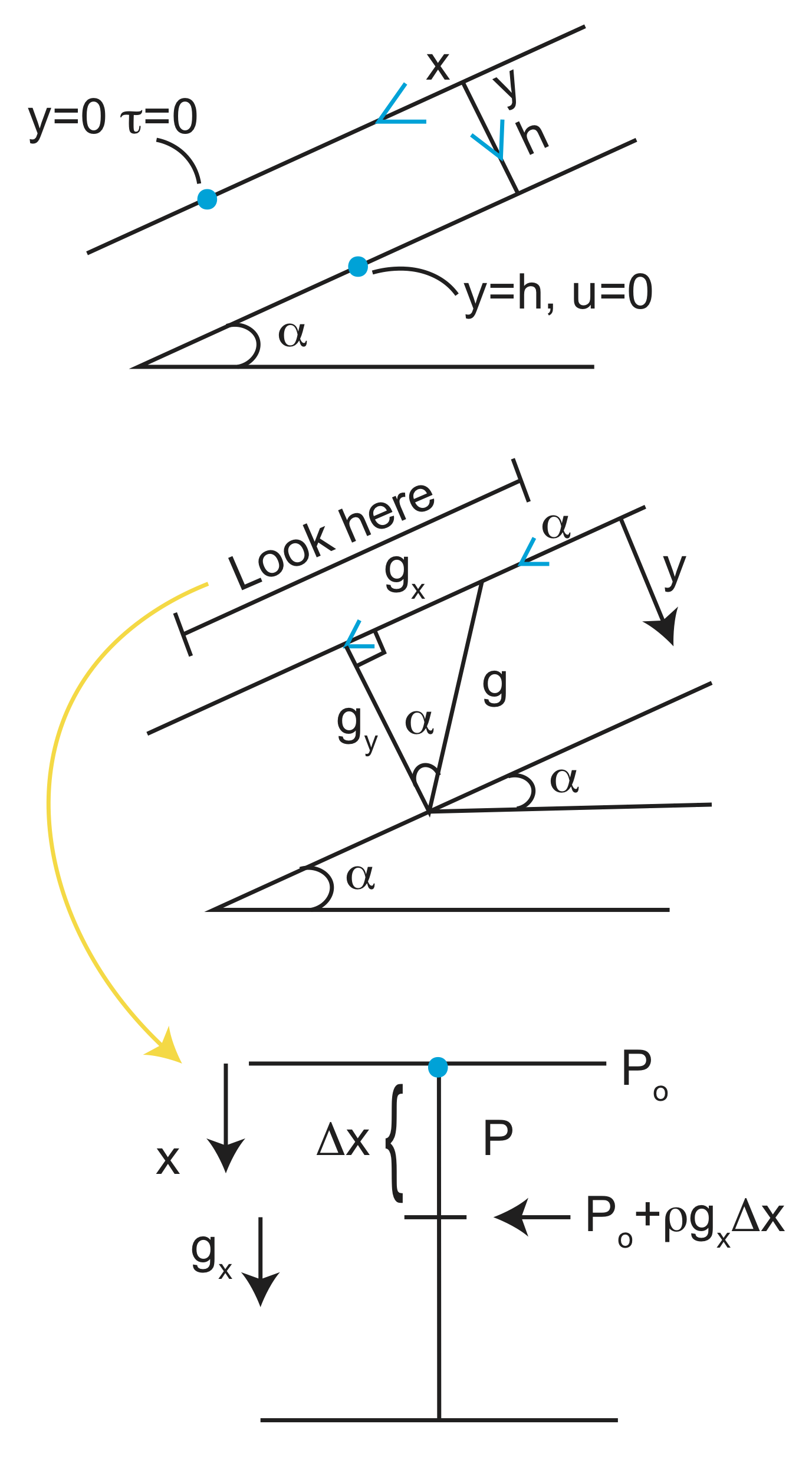
The third panel in the figure below shows how the pressure changes in fluid. At some positions x, the pressure is \(P_o\). At a position \(\Delta x\) down the plane, the pressure is \(P_o +pg\sin(\alpha)\Delta x\) . Therefore, the pressure difference in the fluid is
\[\Delta P=P_o - (P_o +pg\sin(\alpha)\Delta x \nonumber\]
or rearranging to get the pressure gradient
\[\frac{\Delta P}{\Delta x}=-\rho g\sin(\alpha) \nonumber\]
Finally, we get that
\[\frac{dp}{dx}=-\rho g\sin(\alpha) \nonumber\]
Substitute \(\frac{d\tau}{dy}=\frac{dp}{dx}\) into our previous general form of the force balance equation, we can solve to get
\[u=\frac{1}{2\eta} (-\rho g\sin(\alpha))y^2 +c_1 y+c_2 . \nonumber\]
We still need our boundary conditions to solve the equation for the integrations constants.
Using the condition that at y=h, u=0, we find that \(c_1=\frac{\rho g\sin(\alpha)}{2\eta}h\)
Using the condition that at y=0, \(\tau=\eta \frac{du}{dy}=0\) we find that
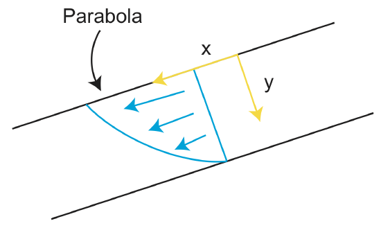
\[ u=\frac{\rho g\sin(\alpha)}{2\eta}(h^2 -y^2) \nonumber\]
Thus, the velocity profile in the inclined plane is a parabola.
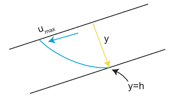
As we can see from the figure, the maximum velocity occurs at the top of the flow, at \(y = 0\).
However, if we use the velocity to determine the strain-rate, we find that
\[ \dot{\epsilon}=\frac{1}{2} \frac{du}{dy}=-\frac{\rho g\sin(\alpha)}{2\eta} y \nonumber\]
Therefore the maximum strain-rate (in terms of magnitude: the sign is not really of importance here) occurs at the bottom of the flow \(y=h\).
This illustrates the important point that fast velocity does not necessarily mean high strain-rate. Instead high strain rate occurs where there is a strong spatial gradient in fluid velocity.