
6.2: Population Growth and Regulation
- Page ID
- 11770
\( \newcommand{\vecs}[1]{\overset { \scriptstyle \rightharpoonup} {\mathbf{#1}} } \)
\( \newcommand{\vecd}[1]{\overset{-\!-\!\rightharpoonup}{\vphantom{a}\smash {#1}}} \)
\( \newcommand{\id}{\mathrm{id}}\) \( \newcommand{\Span}{\mathrm{span}}\)
( \newcommand{\kernel}{\mathrm{null}\,}\) \( \newcommand{\range}{\mathrm{range}\,}\)
\( \newcommand{\RealPart}{\mathrm{Re}}\) \( \newcommand{\ImaginaryPart}{\mathrm{Im}}\)
\( \newcommand{\Argument}{\mathrm{Arg}}\) \( \newcommand{\norm}[1]{\| #1 \|}\)
\( \newcommand{\inner}[2]{\langle #1, #2 \rangle}\)
\( \newcommand{\Span}{\mathrm{span}}\)
\( \newcommand{\id}{\mathrm{id}}\)
\( \newcommand{\Span}{\mathrm{span}}\)
\( \newcommand{\kernel}{\mathrm{null}\,}\)
\( \newcommand{\range}{\mathrm{range}\,}\)
\( \newcommand{\RealPart}{\mathrm{Re}}\)
\( \newcommand{\ImaginaryPart}{\mathrm{Im}}\)
\( \newcommand{\Argument}{\mathrm{Arg}}\)
\( \newcommand{\norm}[1]{\| #1 \|}\)
\( \newcommand{\inner}[2]{\langle #1, #2 \rangle}\)
\( \newcommand{\Span}{\mathrm{span}}\) \( \newcommand{\AA}{\unicode[.8,0]{x212B}}\)
\( \newcommand{\vectorA}[1]{\vec{#1}} % arrow\)
\( \newcommand{\vectorAt}[1]{\vec{\text{#1}}} % arrow\)
\( \newcommand{\vectorB}[1]{\overset { \scriptstyle \rightharpoonup} {\mathbf{#1}} } \)
\( \newcommand{\vectorC}[1]{\textbf{#1}} \)
\( \newcommand{\vectorD}[1]{\overrightarrow{#1}} \)
\( \newcommand{\vectorDt}[1]{\overrightarrow{\text{#1}}} \)
\( \newcommand{\vectE}[1]{\overset{-\!-\!\rightharpoonup}{\vphantom{a}\smash{\mathbf {#1}}}} \)
\( \newcommand{\vecs}[1]{\overset { \scriptstyle \rightharpoonup} {\mathbf{#1}} } \)
\( \newcommand{\vecd}[1]{\overset{-\!-\!\rightharpoonup}{\vphantom{a}\smash {#1}}} \)
\(\newcommand{\avec}{\mathbf a}\) \(\newcommand{\bvec}{\mathbf b}\) \(\newcommand{\cvec}{\mathbf c}\) \(\newcommand{\dvec}{\mathbf d}\) \(\newcommand{\dtil}{\widetilde{\mathbf d}}\) \(\newcommand{\evec}{\mathbf e}\) \(\newcommand{\fvec}{\mathbf f}\) \(\newcommand{\nvec}{\mathbf n}\) \(\newcommand{\pvec}{\mathbf p}\) \(\newcommand{\qvec}{\mathbf q}\) \(\newcommand{\svec}{\mathbf s}\) \(\newcommand{\tvec}{\mathbf t}\) \(\newcommand{\uvec}{\mathbf u}\) \(\newcommand{\vvec}{\mathbf v}\) \(\newcommand{\wvec}{\mathbf w}\) \(\newcommand{\xvec}{\mathbf x}\) \(\newcommand{\yvec}{\mathbf y}\) \(\newcommand{\zvec}{\mathbf z}\) \(\newcommand{\rvec}{\mathbf r}\) \(\newcommand{\mvec}{\mathbf m}\) \(\newcommand{\zerovec}{\mathbf 0}\) \(\newcommand{\onevec}{\mathbf 1}\) \(\newcommand{\real}{\mathbb R}\) \(\newcommand{\twovec}[2]{\left[\begin{array}{r}#1 \\ #2 \end{array}\right]}\) \(\newcommand{\ctwovec}[2]{\left[\begin{array}{c}#1 \\ #2 \end{array}\right]}\) \(\newcommand{\threevec}[3]{\left[\begin{array}{r}#1 \\ #2 \\ #3 \end{array}\right]}\) \(\newcommand{\cthreevec}[3]{\left[\begin{array}{c}#1 \\ #2 \\ #3 \end{array}\right]}\) \(\newcommand{\fourvec}[4]{\left[\begin{array}{r}#1 \\ #2 \\ #3 \\ #4 \end{array}\right]}\) \(\newcommand{\cfourvec}[4]{\left[\begin{array}{c}#1 \\ #2 \\ #3 \\ #4 \end{array}\right]}\) \(\newcommand{\fivevec}[5]{\left[\begin{array}{r}#1 \\ #2 \\ #3 \\ #4 \\ #5 \\ \end{array}\right]}\) \(\newcommand{\cfivevec}[5]{\left[\begin{array}{c}#1 \\ #2 \\ #3 \\ #4 \\ #5 \\ \end{array}\right]}\) \(\newcommand{\mattwo}[4]{\left[\begin{array}{rr}#1 \amp #2 \\ #3 \amp #4 \\ \end{array}\right]}\) \(\newcommand{\laspan}[1]{\text{Span}\{#1\}}\) \(\newcommand{\bcal}{\cal B}\) \(\newcommand{\ccal}{\cal C}\) \(\newcommand{\scal}{\cal S}\) \(\newcommand{\wcal}{\cal W}\) \(\newcommand{\ecal}{\cal E}\) \(\newcommand{\coords}[2]{\left\{#1\right\}_{#2}}\) \(\newcommand{\gray}[1]{\color{gray}{#1}}\) \(\newcommand{\lgray}[1]{\color{lightgray}{#1}}\) \(\newcommand{\rank}{\operatorname{rank}}\) \(\newcommand{\row}{\text{Row}}\) \(\newcommand{\col}{\text{Col}}\) \(\renewcommand{\row}{\text{Row}}\) \(\newcommand{\nul}{\text{Nul}}\) \(\newcommand{\var}{\text{Var}}\) \(\newcommand{\corr}{\text{corr}}\) \(\newcommand{\len}[1]{\left|#1\right|}\) \(\newcommand{\bbar}{\overline{\bvec}}\) \(\newcommand{\bhat}{\widehat{\bvec}}\) \(\newcommand{\bperp}{\bvec^\perp}\) \(\newcommand{\xhat}{\widehat{\xvec}}\) \(\newcommand{\vhat}{\widehat{\vvec}}\) \(\newcommand{\uhat}{\widehat{\uvec}}\) \(\newcommand{\what}{\widehat{\wvec}}\) \(\newcommand{\Sighat}{\widehat{\Sigma}}\) \(\newcommand{\lt}{<}\) \(\newcommand{\gt}{>}\) \(\newcommand{\amp}{&}\) \(\definecolor{fillinmathshade}{gray}{0.9}\)Population ecologists make use of a variety of methods to model population dynamics. An accurate model should be able to describe the changes occurring in a population and predict future changes.
Population Growth
The two simplest models of population growth use deterministic equations (equations that do not account for random events) to describe the rate of change in the size of a population over time. The first of these models, exponential growth, describes theoretical populations that increase in numbers without any limits to their growth. The second model, logistic growth, introduces limits to reproductive growth that become more intense as the population size increases. Neither model adequately describes natural populations, but they provide points of comparison.
Exponential Growth
Charles Darwin, in developing his theory of natural selection, was influenced by the English clergyman Thomas Malthus. Malthus published his book in 1798 stating that populations with abundant natural resources grow very rapidly; however, they limit further growth by depleting their resources. The early pattern of accelerating population size is called exponential growth.
The best example of exponential growth in organisms is seen in bacteria. Bacteria are prokaryotes that reproduce largely by binary fission. This division takes about an hour for many bacterial species. If 1000 bacteria are placed in a large flask with an abundant supply of nutrients (so the nutrients will not become quickly depleted), the number of bacteria will have doubled from 1000 to 2000 after just an hour. In another hour, each of the 2000 bacteria will divide, producing 4000 bacteria. After the third hour, there should be 8000 bacteria in the flask. The important concept of exponential growth is that the growth rate—the number of organisms added in each reproductive generation—is itself increasing; that is, the population size is increasing at a greater and greater rate. After 24 of these cycles, the population would have increased from 1000 to more than 16 billion bacteria. When the population size, N, is plotted over time, a J-shaped growth curve is produced (Figure below).
The bacteria-in-a-flask example is not truly representative of the real world where resources are usually limited. However, when a species is introduced into a new habitat that it finds suitable, it may show exponential growth for a while. In the case of the bacteria in the flask, some bacteria will die during the experiment and thus not reproduce; therefore, the growth rate is lowered from a maximal rate in which there is no mortality. The growth rate of a population is largely determined by subtracting the death rate, D, (number organisms that die during an interval) from the birth rate, B, (number organisms that are born during an interval). The growth rate can be expressed in a simple equation that combines the birth and death rates into a single factor: r. This is shown in the following formula:
\[\text { Population growth } = rN \nonumber \]
Logistic Growth
Extended exponential growth is possible only when infinite natural resources are available; this is not the case in the real world. Charles Darwin recognized this fact in his description of the “struggle for existence,” which states that individuals will compete (with members of their own or other species) for limited resources. The successful ones are more likely to survive and pass on the traits that made them successful to the next generation at a greater rate (natural selection). To model the reality of limited resources, population ecologists developed the logistic growth model.
Carrying Capacity and the Logistic Model
In the real world, with its limited resources, exponential growth cannot continue indefinitely. Exponential growth may occur in environments where there are few individuals and plentiful resources, but when the number of individuals gets large enough, resources will be depleted and the growth rate will slow down. Eventually, the growth rate will plateau or level off (Figure below). This population size, which is determined by the maximum population size that a particular environment can sustain, is called the carrying capacity, or K. Thus, it represents the largest number of individuals that can be supported without harm to the given individual and its environment. In real populations, a growing population often overshoots its carrying capacity, and the death rate increases beyond the birth rate causing the population size to decline back to the carrying capacity or below it. Most populations usually fluctuate around the carrying capacity in an undulating fashion rather than existing right at it.
The formula used to calculate logistic growth adds the carrying capacity as a moderating force in the growth rate. The expression “K – N” is equal to the number of individuals that may be added to a population at a given time, and “K – N” divided by “K” is the fraction of the carrying capacity available for further growth. Thus, the exponential growth model is restricted by this factor to generate the logistic growth equation:
\[\text { Population growth } = rN \left [\dfrac{K-N}{K} \right] \nonumber \]
Notice that when N is almost zero the quantity in brackets is almost equal to 1 (or K/K) and growth is close to exponential. When the population size is equal to the carrying capacity, or N = K, the quantity in brackets is equal to zero and growth is equal to zero. A graph of this equation (logistic growth) yields the S-shaped curve (Figure below). It is a more realistic model of population growth than exponential growth. There are three different sections to an S-shaped curve. Initially, growth is exponential because there are few individuals and ample resources available. Then, as resources begin to become limited, the growth rate decreases. Finally, the growth rate levels off at the carrying capacity of the environment, with little change in population number over time.
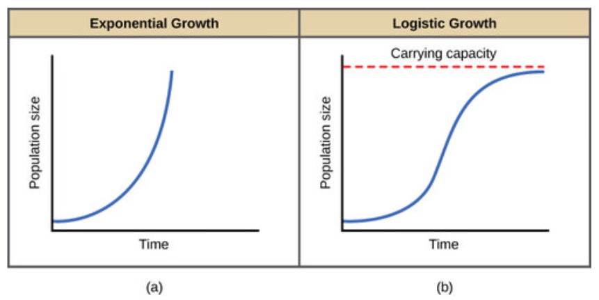 Figure \(\PageIndex{1}\): When resources are unlimited, populations exhibit (a) exponential growth, shown in a J-shaped curve. When resources are limited, populations exhibit (b) logistic growth. In logistic growth, population expansion decreases as resources become scarce, and it levels off when the carrying capacity of the environment is reached. The logistic growth curve is S-shaped.
Role of Intraspecific Competition
The logistic model assumes that every individual within a population will have equal access to resources and, thus, an equal chance for survival. For plants, the amount of water, sunlight, nutrients, and space to grow are the important resources, whereas in animals, important resources include food, water, shelter, nesting space, and mates.
In the real world, phenotypic variation among individuals within a population means that some individuals will be better adapted to their environment than others. The resulting competition for resources among population members of the same species is termed intraspecific competition. Intraspecific competition may not affect populations that are well below their carrying capacity, as resources are plentiful and all individuals can obtain what they need. However, as population size increases, this competition intensifies. In addition, the accumulation of waste products can reduce carrying capacity in an environment.
Examples of Logistic Growth
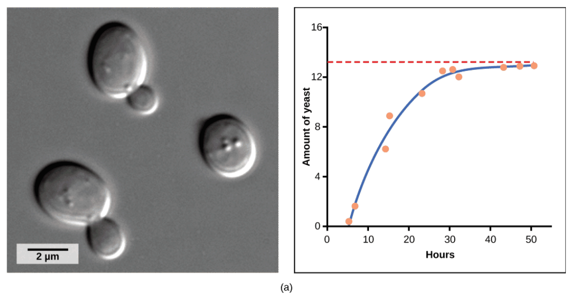
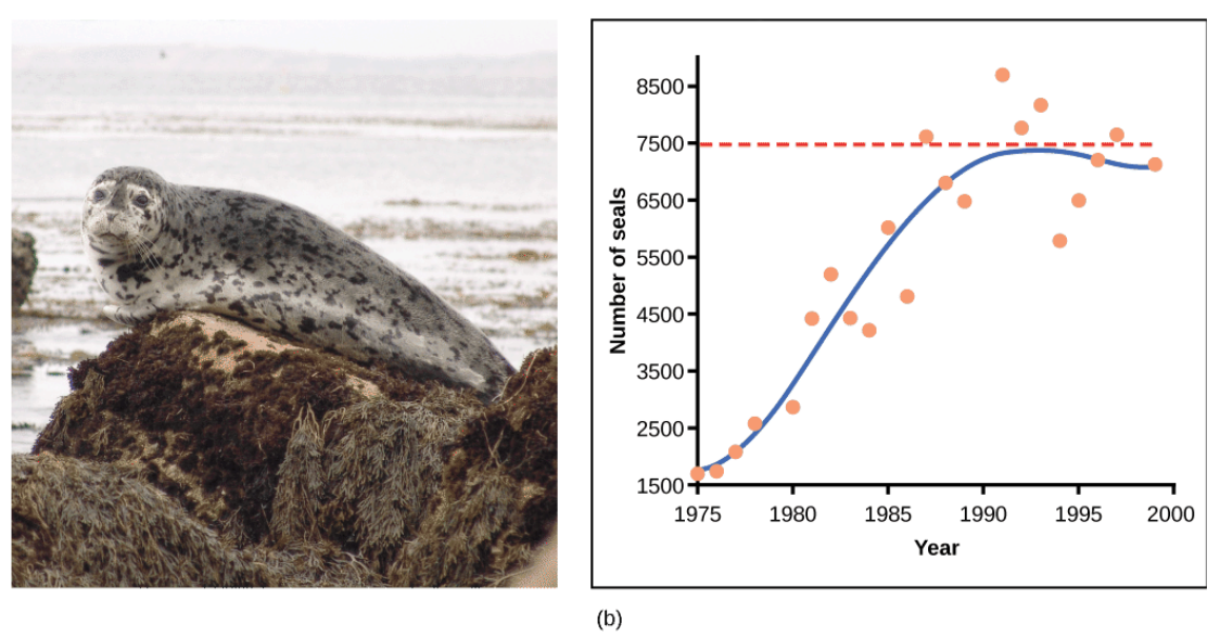
Yeast, a microscopic fungus used to make bread and alcoholic beverages, exhibits the classical S-shaped curve when grown in a test tube (Figure below). Its growth levels off as the population depletes the nutrients that are necessary for its growth. In the real world, however, there are variations to this idealized curve. Examples in wild populations include sheep and harbor seals (Figure below). In both examples, the population size exceeds the carrying capacity for short periods of time and then falls below the carrying capacity afterwards. This fluctuation in population size continues to occur as the population oscillates around its carrying capacity. Still, even with this oscillation, the logistic model is confirmed.
Population Dynamics and Regulation
The logistic model assumes that every individual within a population will have equal access to resources and, thus, an equal chance for survival. For plants, the amount of water, sunlight, nutrients, and space to grow are the important resources, whereas in animals, important resources include food, water, shelter, nesting space, and mates.
In the real world, phenotypic variation among individuals within a population means that some individuals will be better adapted to their environment than others. The resulting competition for resources among population members of the same species is termed intraspecific competition. Intraspecific competition may not affect populations that are well below their carrying capacity, as resources are plentiful and all individuals can obtain what they need. However, as population size increases, this competition intensifies. In addition, the accumulation of waste products can reduce carrying capacity in an environment.
Density-dependent Regulation
Most density-dependent factors are biological in nature and include predation, inter- and intraspecific competition, and parasites. Usually, the denser a population is, the greater its mortality rate. For example, during intra- and interspecific competition, the reproductive rates of the species will usually be lower, reducing their populations’ rate of growth. In addition, low prey density increases the mortality of its predator because it has more difficulty locating its food source. Also, when the population is denser, diseases spread more rapidly among the members of the population, which affect the mortality rate.
Density dependent regulation was studied in a natural experiment with wild donkey populations on two sites in Australia. On one site the population was reduced by a population control program; the population on the other site received no interference. The high-density plot was twice as dense as the low-density plot. From 1986 to 1987 the high-density plot saw no change in donkey density, while the low-density plot saw an increase in donkey density. The difference in the growth rates of the two populations was caused by mortality, not by a difference in birth rates. The researchers found that numbers of offspring birthed by each mother was unaffected by density. Growth rates in the two populations were different mostly because of juvenile mortality caused by the mother’s malnutrition due to scarce high-quality food in the dense population. Figure below shows the difference in age-specific mortalities in the two populations.
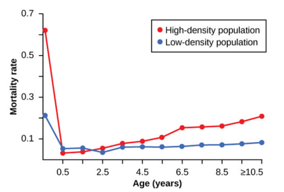 Figure \(\PageIndex{3}\): This graph shows the age-specific mortality rates for wild donkeys from high- and low-density populations. The juvenile mortality is much higher in the high-density population because of maternal malnutrition caused by a shortage of high-quality food.
Density-independent Regulation and Interaction with Density-dependent Factors
Many factors that are typically physical in nature cause mortality of a population regardless of its density. These factors include weather, natural disasters, and pollution. An individual deer will be killed in a forest fire regardless of how many deer happen to be in that area. Its chances of survival are the same whether the population density is high or low. The same holds true for cold winter weather.
In real-life situations, population regulation is very complicated and density-dependent and independent factors can interact. A dense population that suffers mortality from a density-independent cause will be able to recover differently than a sparse population. For example, a population of deer affected by a harsh winter will recover faster if there are more deer remaining to reproduce.
Evolution in Action
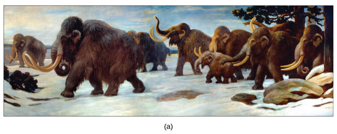
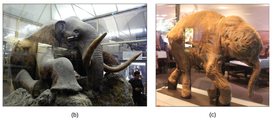 Figure \(\PageIndex{4}\): The three images include: (a) 1916 mural of a mammoth herd from the American Museum of Natural History, (b) the only stuffed mammoth in the world is in the Museum of Zoology located in St. Petersburg, Russia, and (c) a one-month-old baby mammoth, named Lyuba, discovered in Siberia in 2007. (credit a: modification of work by Charles R. Knight; credit b: modification of work by “Tanapon”/Flickr; credit c: modification of work by Matt Howry).
Why did Woolly Mammoth go extinct?
Woolly mammoths began to go extinct about 10,000 years ago, soon after paleontologists believe humans able to hunt them began to colonize North America and northern Eurasia. A mammoth population survived on Wrangel Island, in the East Siberian Sea, and was isolated from human contact until as recently as 1700 BC. We know a lot about these animals from carcasses found frozen in the ice of Siberia and other northern regions. It is commonly thought that climate change and human hunting led to their extinction. A 2008 study estimated that climate change reduced the mammoth’s range from 3,000,000 square miles 42,000 years ago to 310,000 square miles 6,000 years ago. David Nogués-Bravo et al., “Climate Change, Humans, and the Extinction of the Woolly Mammoth.” PLoS Biol 6 (April 2008) Through archaeological evidence of kill sites, it is also well documented that humans hunted these animals. A 2012 study concluded that no single factor was exclusively responsible for the extinction of these magnificent creatures. G.M. MacDonald et al., “Pattern of Extinction of the Woolly Mammoth in Beringia.” Nature Communications 3, no. 893 (June 2012). In addition to climate change and reduction of habitat, scientists demonstrated another important factor in the mammoth’s extinction was the migration of human hunters across the Bering Strait to North America during the last ice age 20,000 years ago. The maintenance of stable populations was and is very complex, with many interacting factors determining the outcome. It is important to remember that humans are also part of nature. Once we contributed to a species’ decline using primitive hunting technology only.
Demographic-Based Population Models
Population ecologists have hypothesized that suites of characteristics may evolve in species that lead to particular adaptations to their environments. These adaptations impact the kind of population growth their species experience. Life history characteristics such as birth rates, age at first reproduction, the numbers of offspring, and even death rates evolve just like anatomy or behavior, leading to adaptations that affect population growth. Population ecologists have described a continuum of life-history “strategies” with K-selected species on one end and r-selected species on the other. K-selected species are adapted to stable, predictable environments. Populations of K-selected species tend to exist close to their carrying capacity. These species tend to have larger, but fewer, offspring and contribute large amounts of resources to each offspring. Elephants would be an example of a K-selected species. r-selected species are adapted to unstable and unpredictable environments. They have large numbers of small offspring. Animals that are r-selected do not provide a lot of resources or parental care to offspring, and the offspring are relatively self-sufficient at birth. Examples of r-selected species are marine invertebrates such as jellyfish and plants such as the dandelion. The two extreme strategies are at two ends of a continuum on which real species life histories will exist. In addition, life history strategies do not need to evolve as suites, but can evolve independently of each other, so each species may have some characteristics that trend toward one extreme or the other.