11.1: How do these fluxes look?
- Page ID
- 6823
\( \newcommand{\vecs}[1]{\overset { \scriptstyle \rightharpoonup} {\mathbf{#1}} } \)
\( \newcommand{\vecd}[1]{\overset{-\!-\!\rightharpoonup}{\vphantom{a}\smash {#1}}} \)
\( \newcommand{\id}{\mathrm{id}}\) \( \newcommand{\Span}{\mathrm{span}}\)
( \newcommand{\kernel}{\mathrm{null}\,}\) \( \newcommand{\range}{\mathrm{range}\,}\)
\( \newcommand{\RealPart}{\mathrm{Re}}\) \( \newcommand{\ImaginaryPart}{\mathrm{Im}}\)
\( \newcommand{\Argument}{\mathrm{Arg}}\) \( \newcommand{\norm}[1]{\| #1 \|}\)
\( \newcommand{\inner}[2]{\langle #1, #2 \rangle}\)
\( \newcommand{\Span}{\mathrm{span}}\)
\( \newcommand{\id}{\mathrm{id}}\)
\( \newcommand{\Span}{\mathrm{span}}\)
\( \newcommand{\kernel}{\mathrm{null}\,}\)
\( \newcommand{\range}{\mathrm{range}\,}\)
\( \newcommand{\RealPart}{\mathrm{Re}}\)
\( \newcommand{\ImaginaryPart}{\mathrm{Im}}\)
\( \newcommand{\Argument}{\mathrm{Arg}}\)
\( \newcommand{\norm}[1]{\| #1 \|}\)
\( \newcommand{\inner}[2]{\langle #1, #2 \rangle}\)
\( \newcommand{\Span}{\mathrm{span}}\) \( \newcommand{\AA}{\unicode[.8,0]{x212B}}\)
\( \newcommand{\vectorA}[1]{\vec{#1}} % arrow\)
\( \newcommand{\vectorAt}[1]{\vec{\text{#1}}} % arrow\)
\( \newcommand{\vectorB}[1]{\overset { \scriptstyle \rightharpoonup} {\mathbf{#1}} } \)
\( \newcommand{\vectorC}[1]{\textbf{#1}} \)
\( \newcommand{\vectorD}[1]{\overrightarrow{#1}} \)
\( \newcommand{\vectorDt}[1]{\overrightarrow{\text{#1}}} \)
\( \newcommand{\vectE}[1]{\overset{-\!-\!\rightharpoonup}{\vphantom{a}\smash{\mathbf {#1}}}} \)
\( \newcommand{\vecs}[1]{\overset { \scriptstyle \rightharpoonup} {\mathbf{#1}} } \)
\( \newcommand{\vecd}[1]{\overset{-\!-\!\rightharpoonup}{\vphantom{a}\smash {#1}}} \)
\(\newcommand{\avec}{\mathbf a}\) \(\newcommand{\bvec}{\mathbf b}\) \(\newcommand{\cvec}{\mathbf c}\) \(\newcommand{\dvec}{\mathbf d}\) \(\newcommand{\dtil}{\widetilde{\mathbf d}}\) \(\newcommand{\evec}{\mathbf e}\) \(\newcommand{\fvec}{\mathbf f}\) \(\newcommand{\nvec}{\mathbf n}\) \(\newcommand{\pvec}{\mathbf p}\) \(\newcommand{\qvec}{\mathbf q}\) \(\newcommand{\svec}{\mathbf s}\) \(\newcommand{\tvec}{\mathbf t}\) \(\newcommand{\uvec}{\mathbf u}\) \(\newcommand{\vvec}{\mathbf v}\) \(\newcommand{\wvec}{\mathbf w}\) \(\newcommand{\xvec}{\mathbf x}\) \(\newcommand{\yvec}{\mathbf y}\) \(\newcommand{\zvec}{\mathbf z}\) \(\newcommand{\rvec}{\mathbf r}\) \(\newcommand{\mvec}{\mathbf m}\) \(\newcommand{\zerovec}{\mathbf 0}\) \(\newcommand{\onevec}{\mathbf 1}\) \(\newcommand{\real}{\mathbb R}\) \(\newcommand{\twovec}[2]{\left[\begin{array}{r}#1 \\ #2 \end{array}\right]}\) \(\newcommand{\ctwovec}[2]{\left[\begin{array}{c}#1 \\ #2 \end{array}\right]}\) \(\newcommand{\threevec}[3]{\left[\begin{array}{r}#1 \\ #2 \\ #3 \end{array}\right]}\) \(\newcommand{\cthreevec}[3]{\left[\begin{array}{c}#1 \\ #2 \\ #3 \end{array}\right]}\) \(\newcommand{\fourvec}[4]{\left[\begin{array}{r}#1 \\ #2 \\ #3 \\ #4 \end{array}\right]}\) \(\newcommand{\cfourvec}[4]{\left[\begin{array}{c}#1 \\ #2 \\ #3 \\ #4 \end{array}\right]}\) \(\newcommand{\fivevec}[5]{\left[\begin{array}{r}#1 \\ #2 \\ #3 \\ #4 \\ #5 \\ \end{array}\right]}\) \(\newcommand{\cfivevec}[5]{\left[\begin{array}{c}#1 \\ #2 \\ #3 \\ #4 \\ #5 \\ \end{array}\right]}\) \(\newcommand{\mattwo}[4]{\left[\begin{array}{rr}#1 \amp #2 \\ #3 \amp #4 \\ \end{array}\right]}\) \(\newcommand{\laspan}[1]{\text{Span}\{#1\}}\) \(\newcommand{\bcal}{\cal B}\) \(\newcommand{\ccal}{\cal C}\) \(\newcommand{\scal}{\cal S}\) \(\newcommand{\wcal}{\cal W}\) \(\newcommand{\ecal}{\cal E}\) \(\newcommand{\coords}[2]{\left\{#1\right\}_{#2}}\) \(\newcommand{\gray}[1]{\color{gray}{#1}}\) \(\newcommand{\lgray}[1]{\color{lightgray}{#1}}\) \(\newcommand{\rank}{\operatorname{rank}}\) \(\newcommand{\row}{\text{Row}}\) \(\newcommand{\col}{\text{Col}}\) \(\renewcommand{\row}{\text{Row}}\) \(\newcommand{\nul}{\text{Nul}}\) \(\newcommand{\var}{\text{Var}}\) \(\newcommand{\corr}{\text{corr}}\) \(\newcommand{\len}[1]{\left|#1\right|}\) \(\newcommand{\bbar}{\overline{\bvec}}\) \(\newcommand{\bhat}{\widehat{\bvec}}\) \(\newcommand{\bperp}{\bvec^\perp}\) \(\newcommand{\xhat}{\widehat{\xvec}}\) \(\newcommand{\vhat}{\widehat{\vvec}}\) \(\newcommand{\uhat}{\widehat{\uvec}}\) \(\newcommand{\what}{\widehat{\wvec}}\) \(\newcommand{\Sighat}{\widehat{\Sigma}}\) \(\newcommand{\lt}{<}\) \(\newcommand{\gt}{>}\) \(\newcommand{\amp}{&}\) \(\definecolor{fillinmathshade}{gray}{0.9}\)
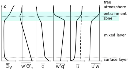
Figure: The mean values and turbulent vertical fluxes of virtual potential temperature, specific humidity, and horizontal momentum for daytime conditions. The top horizontal dashed line indicates the top of the boundary layer; the bottom horizontal dashed line indicates the top of the surface layer. The vertical dashed line is the calculated value of the geostrophic wind extending to the surface if there were no friction. The entrainment zone is an area of mixing between the mixed layer and the free atmosphere. Credit: W. Brune, after Deidonks and Tennekes, 1984
Check Yourself
First, start with some general observations:
- All these height variations scale with the PBL height, whether it be 1 km or 3 km.
- Eddy fluxes move quantities from higher to lower values. If a mean quantity increases with height, then the eddy flux will be downward (negative); if a mean quantity decreases with height, then the eddy flux will be upward (positive).
- The entrainment zone is a layer of mixing between the boundary layer and the free troposphere.
Before you read on, make sure that you believe these three concepts.
Virtual Potential Temperature, \(\bar{\theta}_{v}\)
The \(\bar{\theta}_{v}\) profile is superadiabatic near the surface due to contact with the heated surface, neutral in the middle, and stable above. Eddies can rise from the surface to a height where \(\overline{\boldsymbol{\theta}}_{v}\) equals its surface value (assuming no cloud formation and condensation). The mixed layer will grow if surface heating or increased humidity by evaporation causes the surface \(\bar{\theta}_{v}\) to increase, which means that air parcels can rise and be neutrally buoyant at greater \(\bar{\theta}_{v}\) aloft and thus greater heights.
We see that the eddy flux \(\overline{w^{\prime} \theta}_{v}^{\prime}\) is greatest at the surface, decreases nearly linearly with height, becomes slightly negative above the PBL height h because eddies are bringing warmer air down from above. Remember, eddy fluxes carry a quantity like virtual potential temperature down the mean gradient. The eddy flux for virtual potential temperature (and all quantities) goes to very low values (essentially zero) above the entrainment zone even though a gradient is present because the eddy energy is much lower there.
Specific Humidity, \(\bar{q}\)
Specific humidity is greatest at the surface, where moisture sources, such as water bodies and vegetation, are present. The specific humidity falls off slowly with height until it reaches the PBL height, and then falls off rapidly into the free atmosphere. Because \(\bar{q}\) falls off with height, the humidity flux \(\overline{w^{\prime} q^{\prime}}\) increases with height until \(\overline{w^{\prime} q^{\prime}}\) becomes small because \(\bar{q}\) becomes small.
So what does the daytime convective boundary layer look like? There are isolated convective updrafts surrounded by slower descending air, giving rise to the large-scale eddy circulation, as seen in the following video of the convective boundary layer, viewed from the top. Associated with the large eddies are smaller eddies that come about as the upward and downward air parcels move past each other. If you look closely, you will see eddies of all sizes in the video (:24), some quite large and some quite small, but the smaller ones seem to originate in the larger ones.
Quiz 11-2: State of flux.
- Find Practice Quiz 11-2 in Canvas. You may complete this practice quiz as many times as you want. It is not graded, but it allows you to check your level of preparedness before taking the graded quiz.
- When you feel you are ready, take Quiz 11-2. You will be allowed to take this quiz only once. Good luck!

