
10.10: A Closer Look at the Four Force Balances
- Page ID
- 6550
\( \newcommand{\vecs}[1]{\overset { \scriptstyle \rightharpoonup} {\mathbf{#1}} } \)
\( \newcommand{\vecd}[1]{\overset{-\!-\!\rightharpoonup}{\vphantom{a}\smash {#1}}} \)
\( \newcommand{\id}{\mathrm{id}}\) \( \newcommand{\Span}{\mathrm{span}}\)
( \newcommand{\kernel}{\mathrm{null}\,}\) \( \newcommand{\range}{\mathrm{range}\,}\)
\( \newcommand{\RealPart}{\mathrm{Re}}\) \( \newcommand{\ImaginaryPart}{\mathrm{Im}}\)
\( \newcommand{\Argument}{\mathrm{Arg}}\) \( \newcommand{\norm}[1]{\| #1 \|}\)
\( \newcommand{\inner}[2]{\langle #1, #2 \rangle}\)
\( \newcommand{\Span}{\mathrm{span}}\)
\( \newcommand{\id}{\mathrm{id}}\)
\( \newcommand{\Span}{\mathrm{span}}\)
\( \newcommand{\kernel}{\mathrm{null}\,}\)
\( \newcommand{\range}{\mathrm{range}\,}\)
\( \newcommand{\RealPart}{\mathrm{Re}}\)
\( \newcommand{\ImaginaryPart}{\mathrm{Im}}\)
\( \newcommand{\Argument}{\mathrm{Arg}}\)
\( \newcommand{\norm}[1]{\| #1 \|}\)
\( \newcommand{\inner}[2]{\langle #1, #2 \rangle}\)
\( \newcommand{\Span}{\mathrm{span}}\) \( \newcommand{\AA}{\unicode[.8,0]{x212B}}\)
\( \newcommand{\vectorA}[1]{\vec{#1}} % arrow\)
\( \newcommand{\vectorAt}[1]{\vec{\text{#1}}} % arrow\)
\( \newcommand{\vectorB}[1]{\overset { \scriptstyle \rightharpoonup} {\mathbf{#1}} } \)
\( \newcommand{\vectorC}[1]{\textbf{#1}} \)
\( \newcommand{\vectorD}[1]{\overrightarrow{#1}} \)
\( \newcommand{\vectorDt}[1]{\overrightarrow{\text{#1}}} \)
\( \newcommand{\vectE}[1]{\overset{-\!-\!\rightharpoonup}{\vphantom{a}\smash{\mathbf {#1}}}} \)
\( \newcommand{\vecs}[1]{\overset { \scriptstyle \rightharpoonup} {\mathbf{#1}} } \)
\( \newcommand{\vecd}[1]{\overset{-\!-\!\rightharpoonup}{\vphantom{a}\smash {#1}}} \)
\(\newcommand{\avec}{\mathbf a}\) \(\newcommand{\bvec}{\mathbf b}\) \(\newcommand{\cvec}{\mathbf c}\) \(\newcommand{\dvec}{\mathbf d}\) \(\newcommand{\dtil}{\widetilde{\mathbf d}}\) \(\newcommand{\evec}{\mathbf e}\) \(\newcommand{\fvec}{\mathbf f}\) \(\newcommand{\nvec}{\mathbf n}\) \(\newcommand{\pvec}{\mathbf p}\) \(\newcommand{\qvec}{\mathbf q}\) \(\newcommand{\svec}{\mathbf s}\) \(\newcommand{\tvec}{\mathbf t}\) \(\newcommand{\uvec}{\mathbf u}\) \(\newcommand{\vvec}{\mathbf v}\) \(\newcommand{\wvec}{\mathbf w}\) \(\newcommand{\xvec}{\mathbf x}\) \(\newcommand{\yvec}{\mathbf y}\) \(\newcommand{\zvec}{\mathbf z}\) \(\newcommand{\rvec}{\mathbf r}\) \(\newcommand{\mvec}{\mathbf m}\) \(\newcommand{\zerovec}{\mathbf 0}\) \(\newcommand{\onevec}{\mathbf 1}\) \(\newcommand{\real}{\mathbb R}\) \(\newcommand{\twovec}[2]{\left[\begin{array}{r}#1 \\ #2 \end{array}\right]}\) \(\newcommand{\ctwovec}[2]{\left[\begin{array}{c}#1 \\ #2 \end{array}\right]}\) \(\newcommand{\threevec}[3]{\left[\begin{array}{r}#1 \\ #2 \\ #3 \end{array}\right]}\) \(\newcommand{\cthreevec}[3]{\left[\begin{array}{c}#1 \\ #2 \\ #3 \end{array}\right]}\) \(\newcommand{\fourvec}[4]{\left[\begin{array}{r}#1 \\ #2 \\ #3 \\ #4 \end{array}\right]}\) \(\newcommand{\cfourvec}[4]{\left[\begin{array}{c}#1 \\ #2 \\ #3 \\ #4 \end{array}\right]}\) \(\newcommand{\fivevec}[5]{\left[\begin{array}{r}#1 \\ #2 \\ #3 \\ #4 \\ #5 \\ \end{array}\right]}\) \(\newcommand{\cfivevec}[5]{\left[\begin{array}{c}#1 \\ #2 \\ #3 \\ #4 \\ #5 \\ \end{array}\right]}\) \(\newcommand{\mattwo}[4]{\left[\begin{array}{rr}#1 \amp #2 \\ #3 \amp #4 \\ \end{array}\right]}\) \(\newcommand{\laspan}[1]{\text{Span}\{#1\}}\) \(\newcommand{\bcal}{\cal B}\) \(\newcommand{\ccal}{\cal C}\) \(\newcommand{\scal}{\cal S}\) \(\newcommand{\wcal}{\cal W}\) \(\newcommand{\ecal}{\cal E}\) \(\newcommand{\coords}[2]{\left\{#1\right\}_{#2}}\) \(\newcommand{\gray}[1]{\color{gray}{#1}}\) \(\newcommand{\lgray}[1]{\color{lightgray}{#1}}\) \(\newcommand{\rank}{\operatorname{rank}}\) \(\newcommand{\row}{\text{Row}}\) \(\newcommand{\col}{\text{Col}}\) \(\renewcommand{\row}{\text{Row}}\) \(\newcommand{\nul}{\text{Nul}}\) \(\newcommand{\var}{\text{Var}}\) \(\newcommand{\corr}{\text{corr}}\) \(\newcommand{\len}[1]{\left|#1\right|}\) \(\newcommand{\bbar}{\overline{\bvec}}\) \(\newcommand{\bhat}{\widehat{\bvec}}\) \(\newcommand{\bperp}{\bvec^\perp}\) \(\newcommand{\xhat}{\widehat{\xvec}}\) \(\newcommand{\vhat}{\widehat{\vvec}}\) \(\newcommand{\uhat}{\widehat{\uvec}}\) \(\newcommand{\what}{\widehat{\wvec}}\) \(\newcommand{\Sighat}{\widehat{\Sigma}}\) \(\newcommand{\lt}{<}\) \(\newcommand{\gt}{>}\) \(\newcommand{\amp}{&}\) \(\definecolor{fillinmathshade}{gray}{0.9}\)Geostrophic Balance
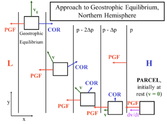
This balance occurs often in atmospheric flow that is a straight line \((R=\pm \infty)\) well above Earth’s surface, so that friction does not matter. The Rossby number, \(R_{O}\), is much less than 1. Let’s think about how this balance might occur. Assume that an air parcel is placed in the midst of a fixed horizontal pressure gradient in the Northern Hemisphere and is initially at rest \((\vec{V}=0)\), as shown in the figure below. The Coriolis force is thus zero and the parcel begins to move from high pressure toward low pressure. However, as the parcel accelerates and attains a velocity perpendicular to the pressure gradient, the Coriolis force begins to increase perpendicular and to the right of the velocity vector and the PGF. The resulting acceleration is now the vector sum of the PGF and the Coriolis forces and turns the parcel to the right. As the velocity continues to increase, the Coriolis force increases but always stays perpendicular and to the right of the velocity vector while the PGF always stays perpendicular to the pressure gradient. Eventually, the PGF and Coriolis force become equal and opposite and the air parcel will move parallel to the horizontal pressure gradient. This condition is called geostrophic balance. We have simplified somewhat the approach to geostrophic equilibrium because, in reality, air parcels would overshoot and undergo inertial oscillations (discussed below) and because the pressure field would evolve in response to the motion.
\[-f V-\frac{\partial \Phi}{\partial n}=0\]geostrophic wind balance
Let the Coriolis force per unit mass be designated as \(C o=-f V\) and the pressure gradient force per unit mass as \(P=-\frac{\partial \Phi}{\partial n}\). Then the force balances are shown in the figure below.
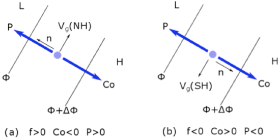
Note that the Coriolis force is always to the right of the velocity vector in the Northern Hemisphere. It is always to the left of the velocity vector in the Southern Hemisphere. When the pressure gradient force and Coriolis force are in balance, the PGF is to the left of the velocity vector and the Coriolis force is to the right in the Northern Hemisphere. Watch the video below (1:10) for further explanation:
Into Geostrophic Balance
- Click here for transcript of the into geostrophic balance video.
-
Let's see how an air partial initially at rest achieves geostrophic balance. At rest, the air parcel velocity equals 0. And the only horizontal force acting on the parcel is the pressure gradient force, which has a constant magnitude and direction as long as the pressure gradient remains the same. As soon as the parcel has some velocity, the Coriolis force starts, perpendicular and to the right of velocity in the northern hemisphere. The Coriolis force begins to move the parcel to the right because the sum of forces on the parcel now has a y component. Note that the PGF is still always perpendicular to the pressure gradient, and the Coriolis force is always perpendicular to the velocity. Eventually, the PGF and the Coriolis force come into opposition with the velocity in between and Coriolis to the right of the velocity. In the end, the y component of the forces is 0 again so that the air parcel remains at the geostrophic velocity.
Inertial Balance
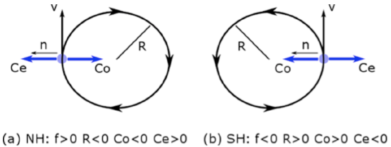
In this case, the pressure gradient force is minimal and the centrifugal and Coriolis forces are in balance.
\[-\frac{V^{2}}{R}-f V=0\]inertial balance
Let the centrifugal force be designated by \(C e=-\frac{V^{2}}{R}\).
We can manipulate Equation [10.37] to find the radius of the circle:
\[R=-\frac{V}{f}\]
For f = 10–4 s–1 and V = 10 m s–1, R = –100 km. Inertial balance is not a major balance in the atmosphere because there is almost always a significant pressure gradient, but it can be important in oceans.
Cyclostrophic Balance
The balance in this case is between the pressure gradient force and the centrifugal force.
\[-\frac{V^{2}}{R}-\frac{\partial \Phi}{\partial n}=0\]
In this case, the scale of the motion is so small that Coriolis acceleration is not important. The Rossby number, Ro = centrifugal acceleration / Coriolis >> 1.
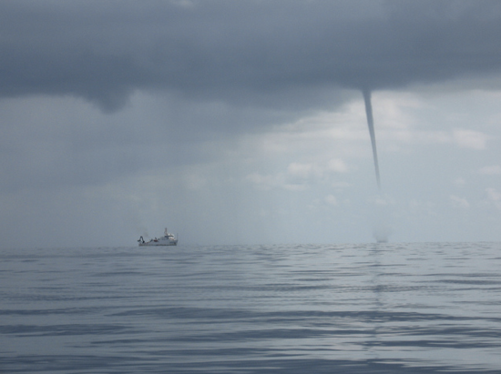
Examples of motion in cyclostrophic balance are tornadoes, dust devils, water spouts, and other small atmospheric circulations, such as the vortex you sometimes see when leaves get swept off the ground. These can be either cyclonic or anticyclonic and, in fact, a few percent of tornadoes in the Northern Hemisphere are anticyclonic. Another common example of cyclostrophic balance is the vortex seen when a bathtub or sink is draining.
Gradient Balance
In gradient balance, the pressure gradient force, Coriolis force, and horizontal centrifugal force are all important. This balance occurs as wind in a pressure gradient field goes around a curve. There are many examples of this type of flow on any weather map—any synoptic-scale pressure gradient for which the isobars curve is an example of gradient flow.
\[-\frac{V^{2}}{R}-f V-\frac{\partial \Phi}{\partial n}=0\]
To solve this equation for velocity, we can use the quadratic equation:
\[a x^{2}+b x+c=0 \quad \rightarrow \quad x=\frac{-b \pm \sqrt{b^{2}-4 a c}}{2 a}\]
\[\frac{V^{2}}{R}+f V+\frac{\partial \Phi}{\partial n}=0 \quad \rightarrow \quad V=\frac{-f \pm \sqrt{f^{2}-4\left(\frac{1}{R}\right) \frac{\partial \Phi}{\partial n}}}{\frac{2}{R}}\]
\[V=-\frac{f R}{2} \pm \sqrt{\frac{f^{2} R^{2}}{4}-R \frac{\partial \Phi}{\partial n}}\]
\(\frac{f^{2} R^{2}}{4}\) is always positive, so, for a given hemisphere (say, the Northern Hemisphere) there are eight possibilities because R can be either positive or negative, \(\frac{\partial \Phi}{\partial n}\) can be positive or negative, and we have the ± sign in between the two terms on the right-hand side of Equation [10.40].
| Northern Hemisphere | R > 0 | R < 0 |
|---|---|---|
| \(\frac{\partial \Phi}{\partial n}>0\) | no roots are physical | only positive root is physical |
| \(\frac{\partial \Phi}{\partial n}<0\) | only positive root is physical | both roots are physical |
The table above gives the results for the Northern Hemisphere (f > 0). We are looking for whether positive or negative values of R and \(\frac{\partial \Phi}{\partial n}\) give non-negative and real values for V because only non-negative and real values for V are physically possible. The reason why real negative values of V are not possible is because the gradient wind balance has been written down in natural coordinates.
- For R > 0 and \(\frac{\partial \Phi}{\partial n}>0\), is always negative, so there are no physical solutions.
- For \(R>0\) and \(\frac{\partial \Phi}{\partial n}<0\), only the plus sign gives a positive V and thus a physical solution.
- For \(R<0\) and \(\frac{\partial \Phi}{\partial n}>0\), only the plus sign gives a positive V and thus a physical solution.
- For \(R<0\) and \(\frac{\partial \Phi}{\partial n}<0\), both roots give positive V and thus physical solutions.
So there are four physical solutions. However, there is one more constraint. This additional constraint is that the absolute angular momentum about the axis of rotation at the latitude of the air parcel should be positive in the Northern Hemisphere (and negative in the Southern Hemisphere). Without proof, we state that only two of the four physically possible cases meet this criterion of positive absolute angular momentum in the Northern Hemisphere. They are:
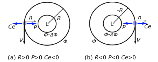
- Regular low: \(R>0\) and \(\frac{\partial \Phi}{\partial n}<0\) and \(V=-\frac{f R}{2}+\sqrt{\frac{f^{2} R^{2}}{4}-R \frac{\partial \Phi}{\partial n}}\)
- Regular high: \(R<0\) and \(\frac{\partial \Phi}{\partial n}<0\) and \(V=-\frac{f R}{2}-\sqrt{\frac{f^{2} R^{2}}{4}-R \frac{\partial \Phi}{\partial n}}\)
These two cases are depicted in the second and third panels of the figure below.
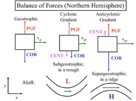
Gradient balance in Northern Hemisphere. left: Geostrophic balance; center: regular low balance; right: regular high balance. Note that the PGF is independent of velocity but both the Coriolis force and the centrifugal force are dependent on velocity. In the figure, vg is used to represent the geostrophic velocity (only the PGF and Coriolis force are important) and vgr is used to represent the gradient wind velocity (the PGF, Coriolis force, and centrifugal force are all important). Credit: H.N. Shirer
The video below ( 3:22) explains these four force balances in more detail:
Four Force Balances
- Click here for transcript of the Four Force Balances video.
-
Let's look at four force balances. Let's start which geostrophic balance, which occurs in straight line flow and [INAUDIBLE] troposphere. In geostrophic flow only the pressure gradient force and the Coriolis force are important. Pressure gradient points to low pressure on the height surface or low height and thus low geopotential on a constant pressure surface is opposed by the Coriolis force which is to the right of the velocity vector in the northern hemisphere and to the left of the velocity vector in the southern hemisphere. Note that we can find the geostrophic velocity if we know the pressure gradient on a constant height surface, or the geopotential or height gradient on a constant pressure surface. For inertial balance the Coriolis force is balanced by the horizontal centrifugal force with the Coriolis force to the right of the velocity vector in the northern hemisphere and to the left in the southern hemisphere. This balance is rarely seen in the atmosphere. Because there's almost always a pressure gradient force of the same magnitude as the centrifugal force and the Coriolis force. In cyclostrophic balance the pressure gradient force is balanced by the centrifugal force. In this case, the velocity vector can be either to the right or to the left of the centrifugal force in both hemispheres. And the Coriolis force is much smaller. This balance is seen in tornadoes and other small vortices. In the northern hemisphere, tornadoes are mostly cyclonic with only a few percent anticyclonic. While smaller vortices are about as often anticyclonic as they are cyclonic. For gradient wind balance the pressure gradient force, Coriolis force, and horizontal centrifugal force are all about equal. To two physical cases are shown for the northern hemisphere in the figure along with the geostrophic balance. With a cyclonic gradient-- that is curvature around the low pressure center-- the PGF points to the low and is constant as long as the pressure gradient is constant. In this case, the PGF is opposed by both the Coriolis force, which depends on the velocity, and the centrifugal force, which depends on the velocity squared. Since the PGF is constant then the sum of the centrifugal and Coriolis force must be equal to it. And since they both depend on velocity the velocity must be less than in the geostrophic case in order for them to be in force balance. This velocity is called subgeostrophic because it is less than the geostrophic velocity. For the anticyclonic gradient-- which is flow around a high-- the PGF points away from the high and is joined by the centrifugal force, which means that the Coriolis force must be stronger than in the geostrophic case because it must balance both the PGF-- which is the same in the geostrophic case-- and the centrifugal force. The Coriolis force can only be greater if the velocity is greater. Thus this velocity is called super geostrophic. Because it is greater than the geostrophic velocity.