7.7: Deformation of Ice

As in many crystals, the way ice crystals are deformed or sheared when a stress is applied is by propagation of dislocations through the crystal. A dislocation is a line defect in a crystal that disrupts the otherwise ideal and regular arrangement of atoms or molecules.

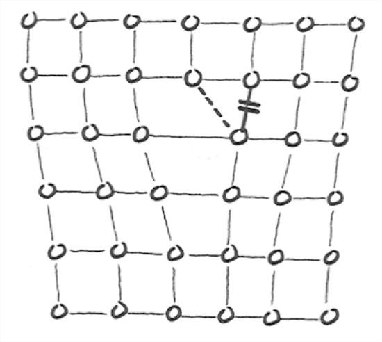
Figure 7-20 shows a simple, idealized example of a dislocation. If we sheared this crystal, the dislocation could migrate simply by breakage of bonds and formation of a new bonds. The net effect is to move the “defected” plane to the right relative to the lower part of the crystal. The dislocation shown in Figure 21 is a line defect that extends indefinitely in one dimension; there are other kinds of dislocations as well.

Ice deforms mainly by propagation of dislocations along the a axis (that’s what the direction perpendicular to the hexagons in the ice structure are called; see the section on ice structure in Chapter 1), so slip is along the basal plane (that is, the plane perpendicular to the a axis). Here’s a loose but not misleading analogy: think of ice as a pack of cards oriented along the basal planes—they’re easy to deform by simple shear along these planes. It’s been shown experimentally that there’s no preferred direction of gliding within the basal plane itself, and it can be demonstrated theoretically that to within a few degrees there shouldn’t be any. There can be gliding by dislocations in nonbasal planes, but that’s much harder—stresses 10–20 times as great are needed—and apparently it’s unimportant.

Figure 7-20. Idealized example of a dislocation.

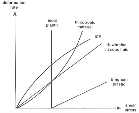
Another way of looking at the nature of deformation of ice is to compare its behavior with other materials in a graph of deformation rate vs. applied shearing stress (Figure 7-21). I mentioned in Chapter 1 that certain fluids, air and water included, show a linear relationship between the applied shearing stress and the rate of shearing deformation. Such fluids are called Newtonian fluids. Fluids that show some other kind of relationship between stress and rate of strain are called non-Newtonian fluids. Ice is one of those. Materials like ice are harder to deform with increasing stress, so that the curve of deformation rate against shear stress is convex upward.

ADVANCED TOPIC: THE FLOW LAW FOR ICE

The relationship between applied stress and rate of deformation for a continuum is called a flow law. What is the flow law for ice? The flow law for ice (both single-crystal and polycrystalline) is of the form

rate of shearing deformation = A (shearing stress)ⁿ (2)

where A is a coefficient and n is an exponent. (In the case of water or air, the exponent n is just 1.)

Figure 7-21. Graph of deformation rate against applied shear stress, showing behavior of various kinds of materials.

In simple shear (Figure 7-22),

\(du\)(3)

Figure 7-22. Definition sketch for analysis of simple shear in glacier ice.

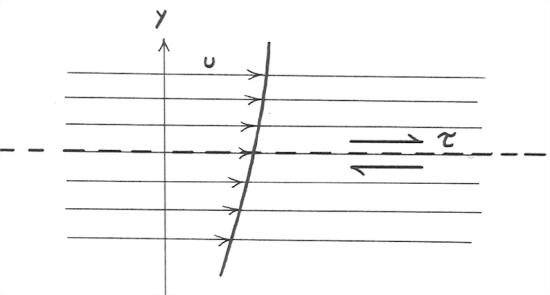
The derivative du/dy, the rate of change of velocity with distance perpendicular to the planes of shearing, is what I referred to above as the rate of shearing deformation. (The coefficient 2 gets there by virtue of the way the rate of deformation is defined; don’t worry about it.) In Equation 3 the coefficient A is like 1/viscosity. It depends strongly on temperature. As you might expect, it’s much smaller (that is, the viscosity is much greater), by two orders of magnitude, for polycrystalline ice than for single-crystal ice oriented with the basal plane parallel to the shear planes. This is because deformation of ice is by internal gliding along the basal planes, and in polycrystalline ice, most crystals are not oriented favorably for this. The exponent n is hard to measure accurately, even in the laboratory! The value usually cited is 3 for polycrystalline ice—but there’s nothing exact about this value. And n doesn’t depend importantly on either temperature or pressure.

ADVANCED TOPIC: THE DOWNSLOPE FLOW OF GLACIERS

One thing we can do by way of theory on glacier movement is to consider the equilibrium of a given reach or streamwise segment of the glacier by writing a force-balance equation. This parallels the derivation of the fundamental resistance equation for rivers in Chapter 5.

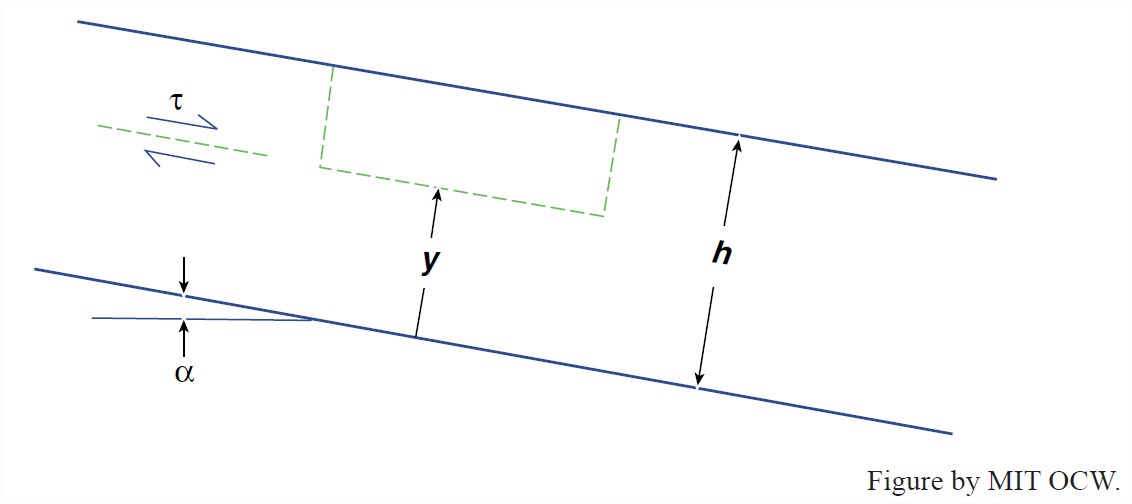
Think about a somewhat idealized glacier of uniform thickness and infinitely wide lateral extent flowing down a planar bedrock surface (Figure 7-23). There must be a balance between the downslope component of gravity (the driving force) and the friction between the glacier and its bed (the resisting force), just as in steady uniform flow of water in an open channel. Accelerations of the glacier are very small and can be ignored for this purpose, although they are not unimportant in other respects.

Figure 7-23. Definition sketch for force balance on a mass of ice in a valley glacier, to derive a resistance equation for glacier flow.

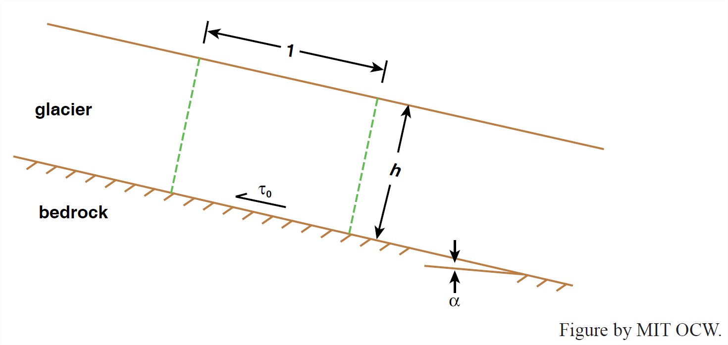
3. Writing the force balance for a block of the glacier with unit width and unit length, as shown in Figure 7-23 (just as for steady uniform channel flow of water; see Chapter 5 on rivers),

\(a_{\tau }= \rho gh sin\alpha\) (4)

where τ_o is the shear stress, ρ is the density of ice, g is the acceleration of gravity, h is the thickness of ice, and α is the slope angle.

Here are two ways Equation 4 is important:

• It provides the best way of estimating the boundary shear stress of a glacier: typically 0.5–1.5 bars (1 bar is approximately 1 atmosphere). Note: this is far smaller than the hydrostatic pressure at the base of the glacier.
• This doesn’t tell us anything about velocities in the glacier. But it can, if we combine it with the flow law for ice. See the following development if you’re interested in the details.

First modify the resistance equation, Equation 4, to get τ as a function of position above the bed (Figure 7-24):

\(\tau = \rho g(h-y)sin\alpha \)(5)

Now we have two equations for τ:

\(\tau ^{n}= \frac{1}{2A}\frac{du}{dy}\)(6)

\( \tau ^{n}=[\rho gsin\alpha (h-y)]^{n}\)(7)

Eliminating τ from Equations 6 and 7,

\(\frac{du}{dy}=2A[\rho g(h-y)sin\alpha ]^{n}\)(8)

This simple differential equation is easy to solve:

\(u = 2A (\rho gsin\alpha )n\int_{0}^{h}(h-y)^{n}dy+c\)(9)

To evaluate the constant of integration c, use the boundary condition that u = u_s, the surface velocity, at y =h. You find that c=u_s. So

\(u_{s}-u = \frac{1}{n+1}2A(\rho gsin\alpha )^{n}(h-y)^{n+1}\)(10)

If u = u_b and y = 0, where u_b is the basal-slip part of the glacier velocity, Equation (10) becomes

\(u_{s}-u_{b} = \frac{1}{n+1}2A(\rho gsin\alpha )^{n}h^{n+1}\)(11)

Using the value of 3 for n, Equations (10) and (11) become

\(u_{s}-u = \frac{A}{2}(\rho gsin\alpha )^{3}(h-y)^{4}\)(12)

\(u_{s}-u_{b} = \frac{A}{2}(\rho gsin\alpha )^{3}h^{4}\)(13)

Figure 7-24. Definition sketch for force balance on a mass of ice in a valley glacier, to derive a velocity distribution along a line normal to the base of the glacier.

Note in Equations 12 and 13 that, other things being equal, glacier velocity varies as the third power of the slope and the fourth power of the thickness.

All of this is for steady uniform flow, but because glaciers have very small accelerations, and to a first approximation they are sheets, it’s not bad. But temperature has a very important effect, through variation of the value of A.

How does a theoretical result like this compare with measured velocities? Not bad. So far, such comparisons have been made only for valley glaciers. (To do so, one has to extend the model slightly to deal with a non- infinitely-wide channel, but that’s straightforward).