
4.8: Summary
- Page ID
- 4687

\( \newcommand{\vecs}[1]{\overset { \scriptstyle \rightharpoonup} {\mathbf{#1}} } \)
\( \newcommand{\vecd}[1]{\overset{-\!-\!\rightharpoonup}{\vphantom{a}\smash {#1}}} \)
\( \newcommand{\dsum}{\displaystyle\sum\limits} \)
\( \newcommand{\dint}{\displaystyle\int\limits} \)
\( \newcommand{\dlim}{\displaystyle\lim\limits} \)
\( \newcommand{\id}{\mathrm{id}}\) \( \newcommand{\Span}{\mathrm{span}}\)
( \newcommand{\kernel}{\mathrm{null}\,}\) \( \newcommand{\range}{\mathrm{range}\,}\)
\( \newcommand{\RealPart}{\mathrm{Re}}\) \( \newcommand{\ImaginaryPart}{\mathrm{Im}}\)
\( \newcommand{\Argument}{\mathrm{Arg}}\) \( \newcommand{\norm}[1]{\| #1 \|}\)
\( \newcommand{\inner}[2]{\langle #1, #2 \rangle}\)
\( \newcommand{\Span}{\mathrm{span}}\)
\( \newcommand{\id}{\mathrm{id}}\)
\( \newcommand{\Span}{\mathrm{span}}\)
\( \newcommand{\kernel}{\mathrm{null}\,}\)
\( \newcommand{\range}{\mathrm{range}\,}\)
\( \newcommand{\RealPart}{\mathrm{Re}}\)
\( \newcommand{\ImaginaryPart}{\mathrm{Im}}\)
\( \newcommand{\Argument}{\mathrm{Arg}}\)
\( \newcommand{\norm}[1]{\| #1 \|}\)
\( \newcommand{\inner}[2]{\langle #1, #2 \rangle}\)
\( \newcommand{\Span}{\mathrm{span}}\) \( \newcommand{\AA}{\unicode[.8,0]{x212B}}\)
\( \newcommand{\vectorA}[1]{\vec{#1}} % arrow\)
\( \newcommand{\vectorAt}[1]{\vec{\text{#1}}} % arrow\)
\( \newcommand{\vectorB}[1]{\overset { \scriptstyle \rightharpoonup} {\mathbf{#1}} } \)
\( \newcommand{\vectorC}[1]{\textbf{#1}} \)
\( \newcommand{\vectorD}[1]{\overrightarrow{#1}} \)
\( \newcommand{\vectorDt}[1]{\overrightarrow{\text{#1}}} \)
\( \newcommand{\vectE}[1]{\overset{-\!-\!\rightharpoonup}{\vphantom{a}\smash{\mathbf {#1}}}} \)
\( \newcommand{\vecs}[1]{\overset { \scriptstyle \rightharpoonup} {\mathbf{#1}} } \)
\(\newcommand{\longvect}{\overrightarrow}\)
\( \newcommand{\vecd}[1]{\overset{-\!-\!\rightharpoonup}{\vphantom{a}\smash {#1}}} \)
\(\newcommand{\avec}{\mathbf a}\) \(\newcommand{\bvec}{\mathbf b}\) \(\newcommand{\cvec}{\mathbf c}\) \(\newcommand{\dvec}{\mathbf d}\) \(\newcommand{\dtil}{\widetilde{\mathbf d}}\) \(\newcommand{\evec}{\mathbf e}\) \(\newcommand{\fvec}{\mathbf f}\) \(\newcommand{\nvec}{\mathbf n}\) \(\newcommand{\pvec}{\mathbf p}\) \(\newcommand{\qvec}{\mathbf q}\) \(\newcommand{\svec}{\mathbf s}\) \(\newcommand{\tvec}{\mathbf t}\) \(\newcommand{\uvec}{\mathbf u}\) \(\newcommand{\vvec}{\mathbf v}\) \(\newcommand{\wvec}{\mathbf w}\) \(\newcommand{\xvec}{\mathbf x}\) \(\newcommand{\yvec}{\mathbf y}\) \(\newcommand{\zvec}{\mathbf z}\) \(\newcommand{\rvec}{\mathbf r}\) \(\newcommand{\mvec}{\mathbf m}\) \(\newcommand{\zerovec}{\mathbf 0}\) \(\newcommand{\onevec}{\mathbf 1}\) \(\newcommand{\real}{\mathbb R}\) \(\newcommand{\twovec}[2]{\left[\begin{array}{r}#1 \\ #2 \end{array}\right]}\) \(\newcommand{\ctwovec}[2]{\left[\begin{array}{c}#1 \\ #2 \end{array}\right]}\) \(\newcommand{\threevec}[3]{\left[\begin{array}{r}#1 \\ #2 \\ #3 \end{array}\right]}\) \(\newcommand{\cthreevec}[3]{\left[\begin{array}{c}#1 \\ #2 \\ #3 \end{array}\right]}\) \(\newcommand{\fourvec}[4]{\left[\begin{array}{r}#1 \\ #2 \\ #3 \\ #4 \end{array}\right]}\) \(\newcommand{\cfourvec}[4]{\left[\begin{array}{c}#1 \\ #2 \\ #3 \\ #4 \end{array}\right]}\) \(\newcommand{\fivevec}[5]{\left[\begin{array}{r}#1 \\ #2 \\ #3 \\ #4 \\ #5 \\ \end{array}\right]}\) \(\newcommand{\cfivevec}[5]{\left[\begin{array}{c}#1 \\ #2 \\ #3 \\ #4 \\ #5 \\ \end{array}\right]}\) \(\newcommand{\mattwo}[4]{\left[\begin{array}{rr}#1 \amp #2 \\ #3 \amp #4 \\ \end{array}\right]}\) \(\newcommand{\laspan}[1]{\text{Span}\{#1\}}\) \(\newcommand{\bcal}{\cal B}\) \(\newcommand{\ccal}{\cal C}\) \(\newcommand{\scal}{\cal S}\) \(\newcommand{\wcal}{\cal W}\) \(\newcommand{\ecal}{\cal E}\) \(\newcommand{\coords}[2]{\left\{#1\right\}_{#2}}\) \(\newcommand{\gray}[1]{\color{gray}{#1}}\) \(\newcommand{\lgray}[1]{\color{lightgray}{#1}}\) \(\newcommand{\rank}{\operatorname{rank}}\) \(\newcommand{\row}{\text{Row}}\) \(\newcommand{\col}{\text{Col}}\) \(\renewcommand{\row}{\text{Row}}\) \(\newcommand{\nul}{\text{Nul}}\) \(\newcommand{\var}{\text{Var}}\) \(\newcommand{\corr}{\text{corr}}\) \(\newcommand{\len}[1]{\left|#1\right|}\) \(\newcommand{\bbar}{\overline{\bvec}}\) \(\newcommand{\bhat}{\widehat{\bvec}}\) \(\newcommand{\bperp}{\bvec^\perp}\) \(\newcommand{\xhat}{\widehat{\xvec}}\) \(\newcommand{\vhat}{\widehat{\vvec}}\) \(\newcommand{\uhat}{\widehat{\uvec}}\) \(\newcommand{\what}{\widehat{\wvec}}\) \(\newcommand{\Sighat}{\widehat{\Sigma}}\) \(\newcommand{\lt}{<}\) \(\newcommand{\gt}{>}\) \(\newcommand{\amp}{&}\) \(\definecolor{fillinmathshade}{gray}{0.9}\)Plate tectonics is a large subject with a great deal of sub topics, which can often make it confusing. It is also one of the most important subjects in modern day geology. Let's review what we've leaned in this chapter to make sure that you completely understand and feel confident with the subject.
Forces Driving Plate Motion
We first discussed how exactly plate tectonics happen, ie what are the forces behind plate movement? The simple answer is convection. Convection can be broken up into 3 sub forces, viscous drag, slab push, and ridge pull. These forces should all balance to 0.
\[F_{ridge-push}+F_{slab-pull}-F_{viscous-drag}=0\]
Viscous drag opposes plate motion and the magnitude of drag under a plate can be represented by
\[|\sigma|=\frac{V_o\eta}{h}\]
For drag on both sides of a plate we have the equation:
\[F_{vis.}=\frac{2V_o\eta_{av}}{h}L_{slab}\]
Another main force a subducting plate will encounter is the slab-pull force. This is the force due to the density contrast between a slab and its surroundings, ie the mass anomaly of the slab in the mantle. This force is represented as:
\[F_{sp}=\Delta m L_{slab} g\]
A final force a subducting plate would experience is the ridge push force. Ridge push results from the elevation of oceanic ridges relative to the seafloor. To determine ridge-push forces we first look at the isostatic balance and the depth of oceans w(t), and second look at the force balance on the plate. Balancing all forces gives us
\[ F_{RP}=F_1-F_2-F_3\]
which will eventually give us
\[F_{RP}=g\kappa t\rho_m\propto(T_m-T_s)(1+\frac{2p_m\propto(T_m-T_s)}{\pi(\rho_m-\rho_w)})\]
Magnetic Anomalies on the Seafloor
The most useful way of determining the age of plates is using magnetic stratigraphy. When sea floor is created at spreading centers magma is emplaced at shallow depth or erupted at the surface to form the crust of the growing plate. Certain minerals in the magma (e.g., magnetite) are sensitive to the Earth's magnetic field. The Earth's magnetic field reverses direction in an a-periodic (non-repeating) pattern, and the oriented minerals act like a bar code or finger print with a distinct pattern associated with different time intervals in the geologic past. Using the Geomagnetic reversal time scale one can determine the age of oceanic crust by measuring the present-day magnetic field, removing the contribution from the current magnetic field, and then analyzing the magnetic "anomalies" that remain.
Determining the spreading rate from the magnetic anomalies is done in several steps. First, just look at the pattern. Are the reversals all similar length or different lengths? Is the pattern symmetric with respect to any point on the profile? This last question is key because a symmetric pattern indicates that there is an active or extinct spreading center in the profile, and therefore, you should only be considering the anomalies on one side of the profile in trying to match the pattern of reversals. Next, try to identify some specific pattern... short-short-long-long-short ... and find a similar pattern in the reference geomagnetic timescale. Once the anomalies are matched, the spreading rate is calculated by noting the start and end time of an anomaly at each end of the profile. Then calculate the time duration between the start or end of the first anomaly and the second anomaly \(\Delta t\) and the distance \(\Delta x\) between these two points on the profile. The spreading rate (velocity) is \( v_s = \frac{\Delta x}{\Delta t}\).
Plates Moving on a Plane
In this section, we learned about how the different types of plate boundaries relate to plate movement.
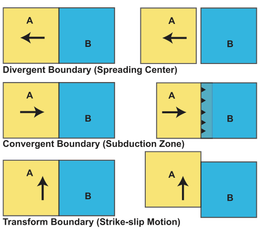
We can see that plate boundary types, in a plate tectonic sense, are defined by the relative velocity of the plates across the boundary. As the forces driving plate motion change, the relative velocity can change. If the change in velocity is large enough it can lead to a change in the type of plate boundary.
Relative Velocity and Reference Frames
Relative velocity is the velocity with respect to some frame of reference. To better understand this, we did several examples with moving and non moving components. Common notation for velocity of an object relative to another object is \( _{fixed} V _{moving} \), or xVy. The question in this case would be what is the motion of object y relative to object x? This can easily be applied to plates, where one is fixed and one is moving. When motion is not directly perpendicular to the plate boundary, it is oblique. The relative velocity in oblique spreading can be determined by first calculating the apparent velocity perpendicular to the ridge, \( V \) and then correcting for the actual orientation of the plate motion given by the angle between the perpendicular direction and the actual plate motion direction \( \alpha \) and is given by
\[ _AV_B = \frac{V}{\cos \alpha} \]
Relative velocity can also be indicated with a velocity line, where regardless of the which plate is held fixed (the reference frame), the relative velocity between to plate is always just the difference in the velocity of the two plates (expressed in the same reference frame). However, plates actually move in two-dimensions (either on a plate or the surface of a sphere). Therefore, to consider relative plate motions and reference frames, we need to deal with the plate velocity as a vector that has both a magnitude and a direction.
\[ V^E = V \sin (\theta) \]
\[V^N = V \cos (\theta) \]
\[V = \sqrt{{V^E}^2 + {V^N}^2} \]
\[ \theta = \tan^{-1} (V^E/V^N) \]
The relative motion of plates in 2D can then be found by adding the components in Cartesian coordinates, and the converting the result to polar coordinates if desired. This process of adding plate velocity vectors can also be illustrated on a velocity plane. Similar to the velocity line the axis represent components of velocity in North and East directions. The velocity vectors are added by drawing the velocity vectors in the appropriate direction and magnitude.
Plate Motions on a Sphere
We then moved on to understanding plate motions of a sphere instead of a plane. Spherical coordinates, as the name suggests, are ideal for dealing with spherical objects. We learned a number of ways to convert between different coordinates including:
- Converting Cartesian to Spherical Coordinates
\[A_x=cos(\lambda)cos(\phi)\]
\[A_y=cos(\lambda)cos(\phi)\]
\[A_z=sin(\lambda)\]
- Converting Spherical to Cartesian Coordinates
\[\lambda=sin^{-1}(A_z)\]
\[\phi=tan^{-1}(\frac{A_y}{A_x})\]
We also learned about the significance of the Euler Pole. A Euler Pole is typically defined by its location (\(\lambda_p,\phi_p\)) and the magnitude of the rotation, \(\omega\), in degrees/my.
To determine angular distance: If given \(\lambda_1, \phi_1\), and \(\lambda_2, \phi_2\)\
- Convert \(\lambda_1, \phi_1\)→\(A_x, A_y, A_z\)
- Convert \(\lambda_2, \phi_2\)→\(B_x, B_y, B_z\)
- Use dot product \(\delta=cos^{-1}(A\cdot B)\)
In Cartesian coordinates, the orientation on x, y, and z are very important. X and y are in the equatorial plane and z points towards the north pole.
Other necessary conversions and variables can be found using known trig relations for triangles on a sphere.