2.5: Darcy's Law - Flow in a Porous Medium
- Page ID
- 3528
\( \newcommand{\vecs}[1]{\overset { \scriptstyle \rightharpoonup} {\mathbf{#1}} } \)
\( \newcommand{\vecd}[1]{\overset{-\!-\!\rightharpoonup}{\vphantom{a}\smash {#1}}} \)
\( \newcommand{\id}{\mathrm{id}}\) \( \newcommand{\Span}{\mathrm{span}}\)
( \newcommand{\kernel}{\mathrm{null}\,}\) \( \newcommand{\range}{\mathrm{range}\,}\)
\( \newcommand{\RealPart}{\mathrm{Re}}\) \( \newcommand{\ImaginaryPart}{\mathrm{Im}}\)
\( \newcommand{\Argument}{\mathrm{Arg}}\) \( \newcommand{\norm}[1]{\| #1 \|}\)
\( \newcommand{\inner}[2]{\langle #1, #2 \rangle}\)
\( \newcommand{\Span}{\mathrm{span}}\)
\( \newcommand{\id}{\mathrm{id}}\)
\( \newcommand{\Span}{\mathrm{span}}\)
\( \newcommand{\kernel}{\mathrm{null}\,}\)
\( \newcommand{\range}{\mathrm{range}\,}\)
\( \newcommand{\RealPart}{\mathrm{Re}}\)
\( \newcommand{\ImaginaryPart}{\mathrm{Im}}\)
\( \newcommand{\Argument}{\mathrm{Arg}}\)
\( \newcommand{\norm}[1]{\| #1 \|}\)
\( \newcommand{\inner}[2]{\langle #1, #2 \rangle}\)
\( \newcommand{\Span}{\mathrm{span}}\) \( \newcommand{\AA}{\unicode[.8,0]{x212B}}\)
\( \newcommand{\vectorA}[1]{\vec{#1}} % arrow\)
\( \newcommand{\vectorAt}[1]{\vec{\text{#1}}} % arrow\)
\( \newcommand{\vectorB}[1]{\overset { \scriptstyle \rightharpoonup} {\mathbf{#1}} } \)
\( \newcommand{\vectorC}[1]{\textbf{#1}} \)
\( \newcommand{\vectorD}[1]{\overrightarrow{#1}} \)
\( \newcommand{\vectorDt}[1]{\overrightarrow{\text{#1}}} \)
\( \newcommand{\vectE}[1]{\overset{-\!-\!\rightharpoonup}{\vphantom{a}\smash{\mathbf {#1}}}} \)
\( \newcommand{\vecs}[1]{\overset { \scriptstyle \rightharpoonup} {\mathbf{#1}} } \)
\( \newcommand{\vecd}[1]{\overset{-\!-\!\rightharpoonup}{\vphantom{a}\smash {#1}}} \)
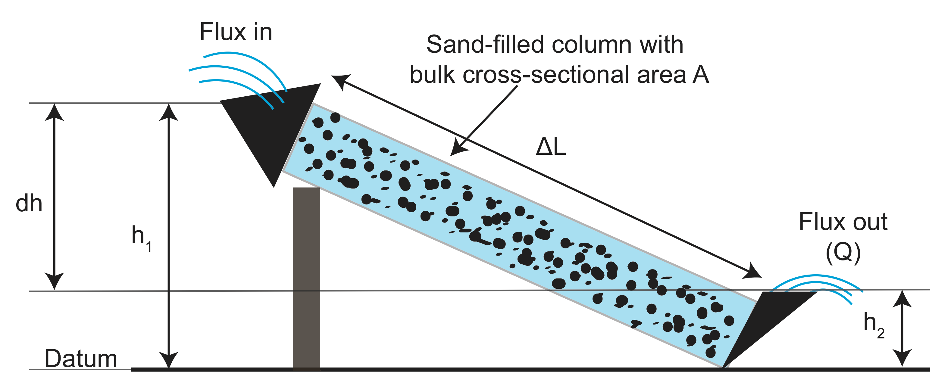
\(\newcommand{\avec}{\mathbf a}\) \(\newcommand{\bvec}{\mathbf b}\) \(\newcommand{\cvec}{\mathbf c}\) \(\newcommand{\dvec}{\mathbf d}\) \(\newcommand{\dtil}{\widetilde{\mathbf d}}\) \(\newcommand{\evec}{\mathbf e}\) \(\newcommand{\fvec}{\mathbf f}\) \(\newcommand{\nvec}{\mathbf n}\) \(\newcommand{\pvec}{\mathbf p}\) \(\newcommand{\qvec}{\mathbf q}\) \(\newcommand{\svec}{\mathbf s}\) \(\newcommand{\tvec}{\mathbf t}\) \(\newcommand{\uvec}{\mathbf u}\) \(\newcommand{\vvec}{\mathbf v}\) \(\newcommand{\wvec}{\mathbf w}\) \(\newcommand{\xvec}{\mathbf x}\) \(\newcommand{\yvec}{\mathbf y}\) \(\newcommand{\zvec}{\mathbf z}\) \(\newcommand{\rvec}{\mathbf r}\) \(\newcommand{\mvec}{\mathbf m}\) \(\newcommand{\zerovec}{\mathbf 0}\) \(\newcommand{\onevec}{\mathbf 1}\) \(\newcommand{\real}{\mathbb R}\) \(\newcommand{\twovec}[2]{\left[\begin{array}{r}#1 \\ #2 \end{array}\right]}\) \(\newcommand{\ctwovec}[2]{\left[\begin{array}{c}#1 \\ #2 \end{array}\right]}\) \(\newcommand{\threevec}[3]{\left[\begin{array}{r}#1 \\ #2 \\ #3 \end{array}\right]}\) \(\newcommand{\cthreevec}[3]{\left[\begin{array}{c}#1 \\ #2 \\ #3 \end{array}\right]}\) \(\newcommand{\fourvec}[4]{\left[\begin{array}{r}#1 \\ #2 \\ #3 \\ #4 \end{array}\right]}\) \(\newcommand{\cfourvec}[4]{\left[\begin{array}{c}#1 \\ #2 \\ #3 \\ #4 \end{array}\right]}\) \(\newcommand{\fivevec}[5]{\left[\begin{array}{r}#1 \\ #2 \\ #3 \\ #4 \\ #5 \\ \end{array}\right]}\) \(\newcommand{\cfivevec}[5]{\left[\begin{array}{c}#1 \\ #2 \\ #3 \\ #4 \\ #5 \\ \end{array}\right]}\) \(\newcommand{\mattwo}[4]{\left[\begin{array}{rr}#1 \amp #2 \\ #3 \amp #4 \\ \end{array}\right]}\) \(\newcommand{\laspan}[1]{\text{Span}\{#1\}}\) \(\newcommand{\bcal}{\cal B}\) \(\newcommand{\ccal}{\cal C}\) \(\newcommand{\scal}{\cal S}\) \(\newcommand{\wcal}{\cal W}\) \(\newcommand{\ecal}{\cal E}\) \(\newcommand{\coords}[2]{\left\{#1\right\}_{#2}}\) \(\newcommand{\gray}[1]{\color{gray}{#1}}\) \(\newcommand{\lgray}[1]{\color{lightgray}{#1}}\) \(\newcommand{\rank}{\operatorname{rank}}\) \(\newcommand{\row}{\text{Row}}\) \(\newcommand{\col}{\text{Col}}\) \(\renewcommand{\row}{\text{Row}}\) \(\newcommand{\nul}{\text{Nul}}\) \(\newcommand{\var}{\text{Var}}\) \(\newcommand{\corr}{\text{corr}}\) \(\newcommand{\len}[1]{\left|#1\right|}\) \(\newcommand{\bbar}{\overline{\bvec}}\) \(\newcommand{\bhat}{\widehat{\bvec}}\) \(\newcommand{\bperp}{\bvec^\perp}\) \(\newcommand{\xhat}{\widehat{\xvec}}\) \(\newcommand{\vhat}{\widehat{\vvec}}\) \(\newcommand{\uhat}{\widehat{\uvec}}\) \(\newcommand{\what}{\widehat{\wvec}}\) \(\newcommand{\Sighat}{\widehat{\Sigma}}\) \(\newcommand{\lt}{<}\) \(\newcommand{\gt}{>}\) \(\newcommand{\amp}{&}\) \(\definecolor{fillinmathshade}{gray}{0.9}\)Darcy's law is crucial to understanding many branches of geology, especially hydrogeology. Before we look at the law and what it can tell us, let's look at how it was developed. Darcy's law is named after Henry Darcy, a 19th century French engineer who developed an underground pressurized pipe system to deliver water around the city of Dijon. The system, which also provided water to the famous Dijon fountains, revolutionized city water and sewage systems. The system required no pumps and was driven purely by gravity. During the process of developing the new system, Darcy conducted a series of experiments where he tried to move water solely using gravity.

From the experiments, collected data on the length of the flume (\(L\)), the cross sectional area of the flume (\(A\)), the height difference (\(h_1 - h_2\)), and the flux of water coming out \(Q\) both with and without granular (filtering) material in the flume. He then plotted the flux measurement normalized by the area versus the ratio of the height difference to the length of the flume (\( \frac{h_1 - h_2}{l}\)). What he found is that there is a linear relationship, and the slope depends on the granular material he used in the flume:
\[\frac{Q}{A}\propto\frac{h_1 - h_2}{L}\]
which can be rewritten as a derivative,
\[Q=-KA\frac{dh}{dx}\]
where \(K\) is the hydraulic conductivity and \(\frac{dh}{dx}\) is the hydraulic gradient. \(Q\), the total discharge rate, has units of \(\frac{m^3}{s}\), the volume of water per time. The negative sign is due to the fact that the fluid flows down (negative) the hydraulic gradient from higher values to lower values.
The hydraulic conductivity is a physical parameter that accounts for how easily the fluid can move through the pore space for the material. In Darcy's original experiments, he used sands with different grain sizes, however, the hydraulic conductivity can be determined for solid rocks as well, as most rocks have some pore space.
Following on Darcy's original experiments, further work was done to understand the physical properties of the fluid and rock that determine the effective hydraulic conductivity. From these experiments it was found that,
\[K = k \frac{\gamma}{\eta} \]
where \(k\) is the intrinsic permeability of the porous media (the solid), \(\eta\) is the dynamic viscosity of the fluid, and \(\gamma = \rho g\) is the specific weight of the fluid, which depends on the fluid density, \(\rho\) and gravity, \(g\).
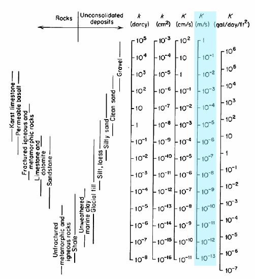
The highlighted column in the figure is K, the hydraulic conductivity in \(\frac{m}{s}\); these are the units that we will be using. The hydraulic conductivity is also sometimes reported in terms of the intrinsic permeability, \(k\), with units of darcys or cm2. The full range of values for hydraulic conductivity is 1-10-13 \(\frac{m}{s}\). Experiments like Darcy's are used to measure K in real materials.

The discharge rate \(Q\) is a volume flux (\(m^3/s\)), but we usually think of fluid flow in terms of a speed or velocity. The discharge questions can be rearranged by dividing through by the area to define the Darcy Flux
\[ q = \frac{Q}{A} = -K \frac{dh}{dx}\; [m/s] \]
Or in terms of the intrinsic permeability and pressure gradient,
\[ q = -\frac{k}{\eta} \frac{dp}{dx} \]
where \(\eta\) is the fluid viscosity (see below for the derivation of the second equation).
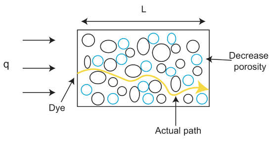
It is important to note that Darcy flux does not equal the fluid velocity, even though it is in units of velocity. The fluid velocity is found through the average linear velocity (\(v_a\)), which is average of the velocity of all possible fluid paths through the porous media: but finding this value is outside the scope of this class. Instead, we will note that the fluid velocity is
\[v=\frac{q}{\varphi}\]
where \(\varphi\) is the porosity and v is the fluid velocity. The porosity, \(\varphi\) is calculated as ratio of the volume of void space to the the total volume of a material \(\varphi=\frac{V_{void}}{V_{tot}}\), and is usually expressed as a fraction between 0 and 1 or as a percent. Note that if \(\varphi\leq\)1 then the fluid velocity is greater the darcy flux.
Another term that arises when discussing flow through rocks and unconsolidated materials is permeability. While porosity is the actual fraction of pores (voids) in the rock, these voids can have different shapes and different connectivity, which affects how easily a fluid can move through the pore space. The permeability is a measure of the ease with which liquids and gases can pass through a rock. The more consolidated the material, the lower its permeability. Thus "loose" materials like gravel have high permeability. Some rocks can also have anisotropic permeability, meaning that fluids can flow easily in one direction, but not in another. An example of a rock with anisotropic permeability is a shale. Fluids can move easily within a layer of the shale, but can not move across layers.

Fluid Velocity
Let's do a basic example.
We are given that \(q=2\frac{m}{min}\) and \(\varphi\) is 25% and want to find the fluid velocity.
We first convert 25% to 0.25.
Then, \(v=\frac{2}{0.25}\frac{m}{min}\)
and
\(v=8 \frac{m}{min}\) is the fluid velocity.
Hydraulic Head
Returning to Darcy's experiments, what is physical process is actually driving the flow of fluid through the flume?
The term \(\frac{dh}{dx} \) is referred to as the hydraulic head, which is the liquid pressure due to the weight of a fluid relative to some reference location: a pressure gradient. However, \(\frac{dh}{dx} \) does not have units of a pressure per unit length, so why is it called the hydraulic head?
Let's consider what the pressure is in the flume in Darcy's experiments. In order to do the experiments, Darcy's had a tank of water at the top end of the flume providing a constant level of water at the top of the flume, equivalent to the height of the flume, \(h_1\). Similarly, there was a tank at the bottom with a constant level of water equivalent to \(h_2\). Therefore the fluid pressure in each of the tanks due to the weight of the water is given by \(P = \rho g h\). The pressure gradient from between the top and the bottom of the plume is then
\[ = \rho g \frac{dh}{dx} \]
or
\[ \frac{dh}{dx} = \frac{1}{\rho g}\frac{dP}{dx} \]
Substituting into Darcy's Law,
\[\begin{align} q&=- K\frac{dh}{dx} \label{Darcy1}\\[4pt] &=\frac{K}{\rho g}\frac{dp}{dx} \end{align}. \]
Recall, from above that the hydraulic conductivity can be written in terms of the intrinsic permeability as \(K = k\frac{\gamma}{\eta}\) which is equivalent to \(k\frac{\rho g}{\eta} \) or rearranging, \(\frac{K}{\rho g} = \frac{k}{\eta} \). Therefore, we can substitute to give two equivalent expressions for Darcy's Law, with one interms of the gradient in height,
\[q=-K\frac{dh}{dx} \]
and the second in terms of the gradient in pressure,
\[ q=\frac{-k}{\eta}\frac{dp}{dx}\]
Thus, \(\frac{dh}{dx}\) is called the hydraulic head because the physical origin of the term in Darcy's Law is the pressure gradient in the fluid, which drives the flow.
Water leaving an Aquifer
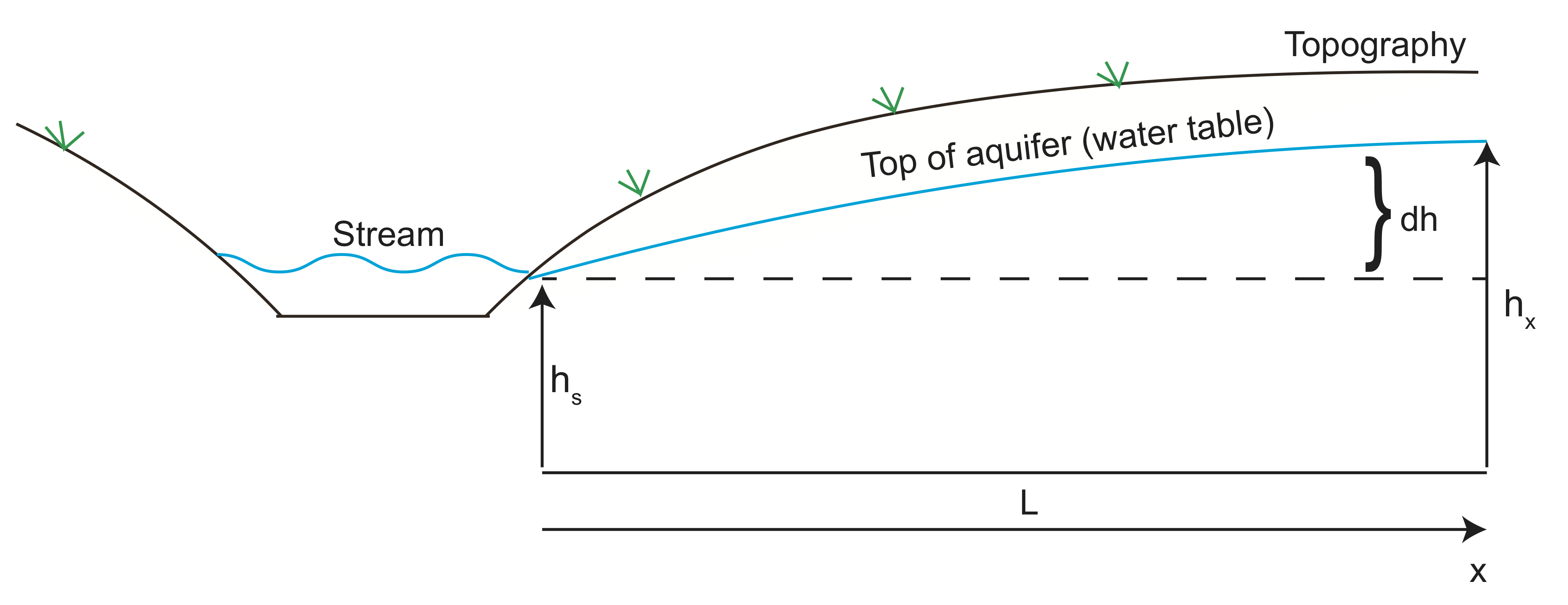
Let's now do an example calculating the fluid velocity of water entering an aquifer. In the sketch below the aquifer height follows the topography on the hill adjacent to the valley with the stream. Water flows from high pressure (head height) toward valley and leaves the aquifer at the stream. We can use Darcy's Law to estimate the rate of water flow form the aquifer.

Using geophysical imaging, the height of the aquifer is found to be 10 m (\(dh\)) above the stream height about 100 meters (\(L\)) away. Assume the hydraulic conductivity is \( K=10^{-6}\) m/s and the porosity is \(\varphi=30\)%.
The darcy flux is
\[q=K \frac{dh}{L} \]
\[q=10^{-6}(\frac{10}{100})\]
\[q =10^{-7}\, \frac{m}{s}\]
The fluid velocity is
\[v=\frac{q}{\varphi}\]
\[v =\frac{10^{-7}}{0.3}\, \text{m/s}\]
\[v =3\times 10^{-8}\, \text{m/s} (3.15\times 10^7 ) \text{s/yr}\]
\[v\approx 0.9\, m/yr\]

Laminar versus Turbulent Flow
One of the implicit assumptions in Darcy's law is that the flow is laminar. Laminar flow is characterized as consisting of thin layers or laminae of fluid all moving parallel to one another. In contrast turbulent flow is characterized by swirls, vortices and eddies, in which adjacent layers of fluid diverge and take different paths down stream.
One way that we can quantify whether a fluid is laminar or turbulent is by calculating the Reynold's number for the flow, defined as
\[Re=\frac{\rho u_oL}{\eta}\; \text{Reynold's number}\]
The Reynold's number is found by considering the two terms in the momentum balance for the flow. The first term is the inertial force per unit volume, which drives the flow, \(\rho u\frac{du}{dx}\). The second term is the viscous force per unit volume, which resists flow, \(\eta\frac{d^2u}{dx^2}\). These two terms must balance, so we can set them equal,
\[\rho u\frac{du}{dx} = \eta\frac{d^2u}{dx^2} \]
Next, we rewrite the terms, in a simplified way to capture only the relevant dimensions of the variables. To do, we go through what is called a dimensional analysis, in which we replace each variable, with a reference values, times a non-dimensional form of the variable.
For example for the term \(x\) is rewritten as just \(L x'\), where \(L\) is the reference length (the fluid depth) and \(x'\) is the non-dimensional distance. Similarly, we let \(u = u_o u'\). Substituting these into the equation, we get
\[\rho u_o \frac{u_o}{L} \frac{du'}{dx'}=\eta\frac{u_o}{L^2} \frac{d^2u'}{dx'^2}\]
Next we combine the constant values out in front
\[\frac{\rho u_oL}{\eta} \frac{du}{dx} = \frac{d^2u}{dx^2} \]
Note that the combination of variables in front is the Reynold's number
\[Re=\frac{\rho u_oL}{\eta}\]
where the variables are \(u_o\) flow velocity, L fluid depth, and the variables we have seen earlier, \(\rho\) fluid density, and \(\eta\) fluid viscosity. By going through this analysis, we find that any flow that is characterized by the balance of these two terms can by compared by simply knowing the value of the Reynolds' number. For example, if one flow has a viscosity that is 10 times the viscosity in another flow, the two flows will behave the same is the density (or velocity or length) is also increased by a factor of 10 for the higher viscosity case; that is, the Reynolds number for the two flows is the same.
To have Darcy flow, the Reynold's number must be less than about 1-10 (laminar). For \(Re>1-10 \) the flow is not strictly laminar, but it is not yet turbulent (non-linear, not-laminar). To have turbulent flow, the Reynold's number must be greater than about 2000.
Understanding that the constants in the numerator and denominator affect the characteristics of the flow in the opposite way, also help to think about how different fluids will behave under similar external conditions. For example, a denser fluid that also has a fast velocity will have a higher Re and exhibit turbulent behavior. In contrast, a fluid such as ice that has a high viscosity and moves very slowly will have a low Re and will likely have laminar flow. The high viscosity of the ice acts to stabilize the flow. As another example, consider two fluids could both be moving at the same velocity behave differently if the other values in the Reynold's number \(\frac{\rho L}{\mu}\) are different. Therefore, the flow type depends not just on the flow velocity, but on the combination of variables in the Reynold's number.
Application of Darcy's Flow
Darcy's law is the main equation that governs flow in aquifers and wells. Without it, we would not be able to drill wells or understand water movement in aquifers, especially in California's central valley, where both these ideas are crucial to both agricultural productivity and groundwater subsidence.


