2.2: Geological Applications of the Diffusion Equation
- Page ID
- 3527
\( \newcommand{\vecs}[1]{\overset { \scriptstyle \rightharpoonup} {\mathbf{#1}} } \)
\( \newcommand{\vecd}[1]{\overset{-\!-\!\rightharpoonup}{\vphantom{a}\smash {#1}}} \)
\( \newcommand{\id}{\mathrm{id}}\) \( \newcommand{\Span}{\mathrm{span}}\)
( \newcommand{\kernel}{\mathrm{null}\,}\) \( \newcommand{\range}{\mathrm{range}\,}\)
\( \newcommand{\RealPart}{\mathrm{Re}}\) \( \newcommand{\ImaginaryPart}{\mathrm{Im}}\)
\( \newcommand{\Argument}{\mathrm{Arg}}\) \( \newcommand{\norm}[1]{\| #1 \|}\)
\( \newcommand{\inner}[2]{\langle #1, #2 \rangle}\)
\( \newcommand{\Span}{\mathrm{span}}\)
\( \newcommand{\id}{\mathrm{id}}\)
\( \newcommand{\Span}{\mathrm{span}}\)
\( \newcommand{\kernel}{\mathrm{null}\,}\)
\( \newcommand{\range}{\mathrm{range}\,}\)
\( \newcommand{\RealPart}{\mathrm{Re}}\)
\( \newcommand{\ImaginaryPart}{\mathrm{Im}}\)
\( \newcommand{\Argument}{\mathrm{Arg}}\)
\( \newcommand{\norm}[1]{\| #1 \|}\)
\( \newcommand{\inner}[2]{\langle #1, #2 \rangle}\)
\( \newcommand{\Span}{\mathrm{span}}\) \( \newcommand{\AA}{\unicode[.8,0]{x212B}}\)
\( \newcommand{\vectorA}[1]{\vec{#1}} % arrow\)
\( \newcommand{\vectorAt}[1]{\vec{\text{#1}}} % arrow\)
\( \newcommand{\vectorB}[1]{\overset { \scriptstyle \rightharpoonup} {\mathbf{#1}} } \)
\( \newcommand{\vectorC}[1]{\textbf{#1}} \)
\( \newcommand{\vectorD}[1]{\overrightarrow{#1}} \)
\( \newcommand{\vectorDt}[1]{\overrightarrow{\text{#1}}} \)
\( \newcommand{\vectE}[1]{\overset{-\!-\!\rightharpoonup}{\vphantom{a}\smash{\mathbf {#1}}}} \)
\( \newcommand{\vecs}[1]{\overset { \scriptstyle \rightharpoonup} {\mathbf{#1}} } \)
\( \newcommand{\vecd}[1]{\overset{-\!-\!\rightharpoonup}{\vphantom{a}\smash {#1}}} \)
\(\newcommand{\avec}{\mathbf a}\) \(\newcommand{\bvec}{\mathbf b}\) \(\newcommand{\cvec}{\mathbf c}\) \(\newcommand{\dvec}{\mathbf d}\) \(\newcommand{\dtil}{\widetilde{\mathbf d}}\) \(\newcommand{\evec}{\mathbf e}\) \(\newcommand{\fvec}{\mathbf f}\) \(\newcommand{\nvec}{\mathbf n}\) \(\newcommand{\pvec}{\mathbf p}\) \(\newcommand{\qvec}{\mathbf q}\) \(\newcommand{\svec}{\mathbf s}\) \(\newcommand{\tvec}{\mathbf t}\) \(\newcommand{\uvec}{\mathbf u}\) \(\newcommand{\vvec}{\mathbf v}\) \(\newcommand{\wvec}{\mathbf w}\) \(\newcommand{\xvec}{\mathbf x}\) \(\newcommand{\yvec}{\mathbf y}\) \(\newcommand{\zvec}{\mathbf z}\) \(\newcommand{\rvec}{\mathbf r}\) \(\newcommand{\mvec}{\mathbf m}\) \(\newcommand{\zerovec}{\mathbf 0}\) \(\newcommand{\onevec}{\mathbf 1}\) \(\newcommand{\real}{\mathbb R}\) \(\newcommand{\twovec}[2]{\left[\begin{array}{r}#1 \\ #2 \end{array}\right]}\) \(\newcommand{\ctwovec}[2]{\left[\begin{array}{c}#1 \\ #2 \end{array}\right]}\) \(\newcommand{\threevec}[3]{\left[\begin{array}{r}#1 \\ #2 \\ #3 \end{array}\right]}\) \(\newcommand{\cthreevec}[3]{\left[\begin{array}{c}#1 \\ #2 \\ #3 \end{array}\right]}\) \(\newcommand{\fourvec}[4]{\left[\begin{array}{r}#1 \\ #2 \\ #3 \\ #4 \end{array}\right]}\) \(\newcommand{\cfourvec}[4]{\left[\begin{array}{c}#1 \\ #2 \\ #3 \\ #4 \end{array}\right]}\) \(\newcommand{\fivevec}[5]{\left[\begin{array}{r}#1 \\ #2 \\ #3 \\ #4 \\ #5 \\ \end{array}\right]}\) \(\newcommand{\cfivevec}[5]{\left[\begin{array}{c}#1 \\ #2 \\ #3 \\ #4 \\ #5 \\ \end{array}\right]}\) \(\newcommand{\mattwo}[4]{\left[\begin{array}{rr}#1 \amp #2 \\ #3 \amp #4 \\ \end{array}\right]}\) \(\newcommand{\laspan}[1]{\text{Span}\{#1\}}\) \(\newcommand{\bcal}{\cal B}\) \(\newcommand{\ccal}{\cal C}\) \(\newcommand{\scal}{\cal S}\) \(\newcommand{\wcal}{\cal W}\) \(\newcommand{\ecal}{\cal E}\) \(\newcommand{\coords}[2]{\left\{#1\right\}_{#2}}\) \(\newcommand{\gray}[1]{\color{gray}{#1}}\) \(\newcommand{\lgray}[1]{\color{lightgray}{#1}}\) \(\newcommand{\rank}{\operatorname{rank}}\) \(\newcommand{\row}{\text{Row}}\) \(\newcommand{\col}{\text{Col}}\) \(\renewcommand{\row}{\text{Row}}\) \(\newcommand{\nul}{\text{Nul}}\) \(\newcommand{\var}{\text{Var}}\) \(\newcommand{\corr}{\text{corr}}\) \(\newcommand{\len}[1]{\left|#1\right|}\) \(\newcommand{\bbar}{\overline{\bvec}}\) \(\newcommand{\bhat}{\widehat{\bvec}}\) \(\newcommand{\bperp}{\bvec^\perp}\) \(\newcommand{\xhat}{\widehat{\xvec}}\) \(\newcommand{\vhat}{\widehat{\vvec}}\) \(\newcommand{\uhat}{\widehat{\uvec}}\) \(\newcommand{\what}{\widehat{\wvec}}\) \(\newcommand{\Sighat}{\widehat{\Sigma}}\) \(\newcommand{\lt}{<}\) \(\newcommand{\gt}{>}\) \(\newcommand{\amp}{&}\) \(\definecolor{fillinmathshade}{gray}{0.9}\)In this section we introduce two applications of the diffusion equation to heat transport, followed by applications to erosion of a fault scarp and diffusive transport of a chemical species (atoms or molecules).
For each of the applications we use the 1-D diffusion equation and the solution is found by defining an initial condition (the initial temperature, topography, or concentration at every position) and two boundary conditions (the value of the temperature, topography, or concentration at two points at either end of the 1-D profile) The boundary conditions can be fixed (constant) in time or change as a function of time. We will go over these conditions in more detail in the next few sections. These initial and boundary conditions, allow us to integrate the differential equations and determine the unknown constants of integration. Because there is one temperature derivative, we need one initial (time) constraint to determine the one constant of integration. Likewise, because there are two derivatives in space, we need two boundary (spatial) conditions to find the two constants of integration.
First, we will go through the a few details related to solving the diffusion equations with these initial and boundary conditions to obtain the temperature profile as a function of time for the specific example of cooling of the oceanic lithosphere. For the other examples, we won't go through all the details, but rather point out the specific differences that arise due to the different boundary conditions.
General Approach to Solving the 1-D Diffusion Equation
We begin with the 1-D diffusion equation for temperature
\[\frac{dT}{dt}=\kappa\frac{d^2T}{dz^2}\]
where \(\kappa\) is the thermal diffusivity. The solution for this equation is:
\[T(x, t)=(T_s-T_m)erfc(\frac{y}{2\sqrt{\kappa t}})+T_m\]
where \(T_s\) is the surface temperature, \(T_m\) is the mantle temperature, and y is the depth into the lithosphere (\(y=0\) at the surface). This is a commonly used thermal profiles when considering the thermal structure of the oceanic lithosphere through purely conductive processes. It does not take into account reheating due to volcanism, radiogenic heating or mechanical feedback, but it is used to define the initial condition in many calculations or numerical simulations including the thermal structure of the lithosphere. We will use it later on to calculate the ridge push force.
Directly solving the partial differential equations (PDE) is beyond the scope of this text, but understanding that the boundary and initial conditions determine how the solution to a specific diffusion problem will look is valuable for considering each of these physical processes and gaining insight into the geological problem.
\[\frac{dT}{dt}=\kappa\frac{d^2T}{dz^2}\]
The term on the left side, \(\frac{dT}{dt}\) takes the derivative of \(T\) in terms of t and holds x constant. Remember from your calculus class, that when we integrate for each derivative there will have a constant of integration. The same is true for solving a PDE. So, from the left side of the equation there will be a constant of integration related to the time derivative. Likewise, on the right-hand side, we have the second derivative of temperature with respect to depth, so there will be two constants of integration. As stated above, the initial condition and the boundary conditions provide the information needed to determine these constants.
- Initial Condition (IC): the starting value for the quantity you are calculating (e.g., temperature) at every point along your profile? This might be a constant or a function of position.
- Boundary Conditions (BCs): the value for the quantity you are calculating e.g., temperature) at each end of your profile (or at infinity depending on the specific problem) for ALL times? These values might be constants or a function of time.
In addition to the IC and BCs, we need to know the values of the physical quantities that show up in our equation. For the diffusion equation, the only constant is the diffusivity, and we need to know this value.
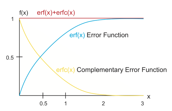
For almost every diffusion equation you come upon, the solution to the equation will include some sort of dependence on the error function, which is defined as,
\[erf(\eta)=\frac{2}{\sqrt{\pi}} \int_{0}^{\eta} e^{-\eta^{\prime 2}} d\eta\prime\]
The parameter \(\eta\) depends on the distance, time, and the diffusion coefficient,
\[\eta=\frac{z}{2\sqrt{\kappa t}}.\]
Note that if you set your \(\eta=1\), you are back to the simple equation that we used to determine the length-scale and time-scale for diffusion. The value of the error function for any particular value of \(\eta\) can be calculated using a built-in function or looked up in a table. There is also a related function called the complementary error function,
\[erfc(\eta)=1-erf(\eta)\]
Application 1: Cooling of a Lithospheric Plate
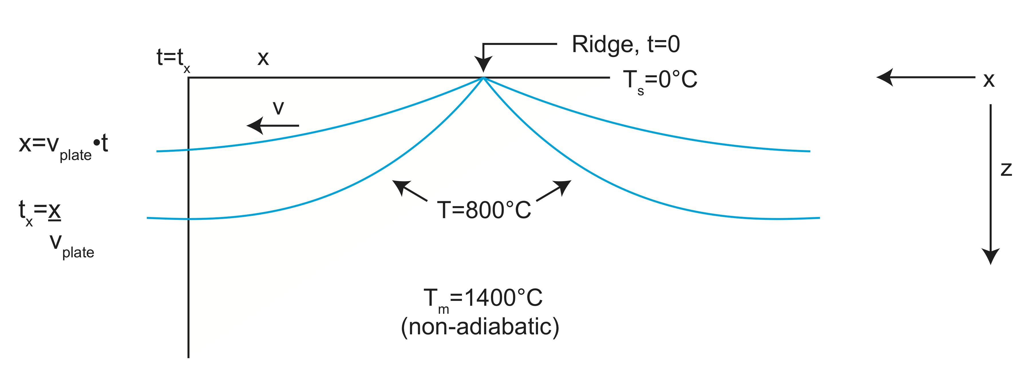
Lithosphere forms by cooling of the mantle as the tectonic plate moves away from a spreading ridge. At the ridge, the mantle temperature of \(T_m\) almost reaches the surface (z=0). As the material formed at the ridge moves away from the spreading center at a rate equal to the speed of the tectonic plate (\(u\)), the mantle cools from above to become the lithosphere. The temperature at the surface of the lithosphere, \(T_s\), is essentially constant because the surface is at the bottom of the ocean (\(T=0^oC)\). The age of the plate at a distance \(x\) from the spreading center is determined by the speed of the plate: \(t=\frac{x}{u}\). A typical value for the thermal diffusion coefficient (thermal diffusivity) is \(\kappa_T=1.0 \times 10^{-6}\frac{m^2}{s}\).
What is the initial condition for the temperature?
At time t=0, the temperature is equal to the mantle temperature at all positions in z, \(T(z, t=0)=T_m\). This is even true at the surface. The temperature at the surface changes to zero at the instant of time just after t=0.
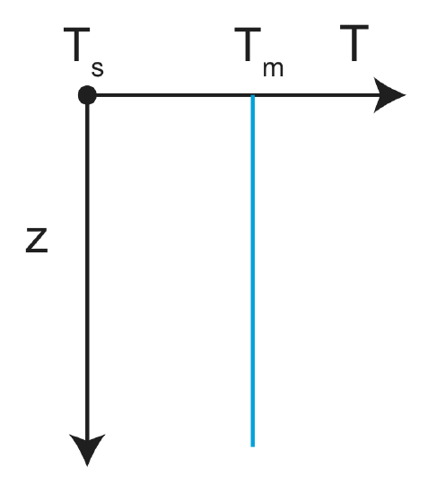
Figure \(\PageIndex{2}\): Initial conditions: \(T(z)=T_s\) at \(z=0\) and \(T(z) = T_m \) for \(z>0\)
What are the boundary conditions for the temperature?
The temperature far away from the surface will stay at the mantle temperature, Tm, and the surface temperature will stay at Ts=0. At z=0, T(0,t)=Ts. As \(z\rightarrow\infty\), T=Tm. Put in another way:
at t=0 T(z=0)=\(T_m\) and, at z=0 T(t>0)=\(T_s\)
t=\(0_+\) T(z=0)=\(T_s\) z=\(\infty\) T(t>0)=\(T_m\)
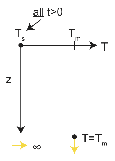
Figure \(\PageIndex{2}\): Boundary conditions: \(T=T_s\) at z = 0 for all \(t>0\) and \(T = T_m\) at \(z = \infty\)
What is \(\eta\) in the error function equation?
\[\eta=\frac{x}{2\sqrt{\kappa t}}\]
Solution
\[T(x, t)=(T_s-T_m) erfc(\frac{x}{2\sqrt{\kappa t}})+T_m\]
We can also rewrite this in terms of \(erf\) instead of \(erfc\) as
\[ \begin{align*} erfc(\eta) &=(1-erf(\eta)) \\[4pt] &=(T_s-T_m)(1-erf(\eta))+T_m \\[4pt] &=(T_s-T_m)-(T_s-T_m)erf(\eta)+T_m \\[4pt] &=T_s-(T_s-T_m)erf(\eta) \\[4pt] &=T_s+(T_m-T_s)erf(\eta) \end{align*}\]
Application 2: Fault Scarp Erosion
The change in shape of a fault scarp profile as a function of time due to erosional processes is often modeled using the diffusion equation. In this case the topography (mass) diffuses (erodes) from the uplifted block to the down-dropped block. For the case of an initial vertical offset, as the diffusive erosion progresses the sharp discontinuity in surface topography will become smoother with the slope across the fault with decreasing time.
For this example, we will consider a 1-D topography profile across a fault with total vertical offset \(\Delta H(x=0)=2a\), and \(H_{x_{max}}=a\) and \(H_{x_{min}}=-a\). The fault could occur in a region with an overall background slope given by b (units of \(\frac{m}{km}\); b=0 is a flat surface). The diffusion coefficient for topography will depend on the type of rock forming the fault and surface processes. Typical diffusion coefficient values are: \(\kappa_H=0.5-1.0 \frac{m^2}{kyr}\), which is \(\kappa_H=1.5-3.0\) x10-11 \(\frac{m^2}{s}\).

What is the initial condition for topography?
At time t=0, the fault has just formed so the topography on either side of the fault has a specified value. For a flat background surface:
At t=0 and \(x\leq 0, H(x)=a\) or \(H(x)=a+bx\)
At t=0 and \(x>0, H(x)=-a\) or \(H(x)=-a-bx\)
What are the boundary conditions for the topography?
For the fault scarp diffusion problem, erosion will only modify the topography in the region near the fault. Far away from the fault, the total offset will not change from the initial value:
As \(x\rightarrow -\infty\), for x\(\leq 0\), \(H(x, t)\rightarrow a+bx\)
As \(x\rightarrow \infty\), for x\(> 0\), \(H(x, t)\rightarrow -a-bx\)
What is \(\eta\) in the error function equation?
\[\eta=\frac{x}{2\sqrt{\kappa_H t}}\]
For the case of erosion of a fault scarp with initial height, H, the diffusion equation can be written as:
\[\frac{\partial H}{\partial t}=\kappa_H(\frac{\partial^2H}{\partial x^2})\]
where \(\kappa_H\) is the diffusivity for fault scarp topography.
Solution
Using the initial and boundary conditions the diffusion equation can be solved for the change in shape of the topography as a function of time and position:
\[H(x, t)=erf(\frac{x}{2\sqrt{\kappa_H t}})a+bx\]
where \(a\) is half the total fault offset and \(b\) is the background slope of topography.
Application 3: Diffusion of Chemical Species (a Solute in Water)
Contamination of groundwater by toxic spills can be modeled as a diffusive process, where the concentration of a toxic substance diffuses out away from the source due to a chemical gradient. Basically, the toxin wants to move form a region of high concentration to a region of low concentration in order to minimize the total energy of the system (thermodynamics concept).
For this example imagine there is a gasoline station with a leaking subsurface gasoline storage compartment. The rate of leakage is constant, so at the position of the leak there is a constant input value of toxin per volume, or constant concentration, Cs (s-spill). Far away from the leak, the concentration is zero (or in general some background value, Co, depending on the solute of interest). For a 1-D profile, with the leakage located at x=0, the diffusion equation can be used to determine how the concentration of the toxin changes with time and distance away from the leakage. The diffusion coefficient for toxins will depend on the type of toxin, the medium it is diffusing through (groundwater in this example) and temperature. Typical concentration diffusion coefficients (\(\kappa_C\)), in groundwater at \(T=25^oC\), are: MTBE (Methyl tert-butyl ether, in gasoline) 9.4x10⁻¹⁰\(\frac{m^2}{s}\), Benzene (in gasoline) 1.1x10⁻⁹\(\frac{m^2}{s}\), and Methanol 1.65x10⁻⁹ \(\frac{m^2}{s}\).
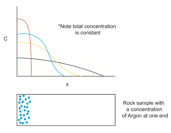
What is the initial condition for the solute concentration?
At time t=0, the leakage starts, so the concentration at x=0 is C=Cs. Elsewhere the concentration is equal to the background value. But also note that at all times C=Cs since the spill continues at a constant rate.
What are the boundary conditions for the solute concentration?
Far away from the leakage, the concentration will be unaffected by the leakage: As \(x\rightarrow\pm\infty\), C=Co (this is in fact two boundary conditions at plus and minus infinity). However, in addition, at the location of the spill the concentration stays constant because the leakage continues at a constant rate: C=Cs at x=0 for all times.
What is \(\eta\) in the error function equation?
\[\eta=\frac{x}{2\sqrt{\kappa_C t}}\]
For the case of diffusion of some chemical element denoted by C, the diffusion equation can be written as:
\[\frac{\partial C}{\partial t}=\kappa_C(\frac{\partial^2C}{\partial x^2})\]
where \(\kappa_C\) is the diffusivity of the chemical element and \(C\) is the concentration of the chemical element.
Solution
Using the initial and boundary conditions the diffusion equation can be solved for the change in concentration of the toxin in the groundwater as a function of time and position
\[C(x, t)=(C_s-C_o)erfc(\frac{x}{2\sqrt{\kappa_C t}})+C_o\]


