1.6: The Flow of Water

1.6.1 Introduction

Much of what happens by way of natural processes on the earth’s surface involves the flow of water or air. Just think about it: the obvious examples are streams and rivers, ocean currents, and the wind. Less obvious, but extremely important, is the flow of groundwater beneath the Earth’s surface. The topic of fluid flow is of central importance in this course, and I would be remiss in not subjecting you to some basic ideas in the dynamics of fluid flow. Of course, whole courses can be devoted to fluid dynamics, and a genuinely deep understanding necessitates much more math and physics than is appropriate for this course. I know, however, from my own experience in teaching fluid dynamics that most of the really important concepts can be made clear without heavy mathematics.

In this section we’ll concentrate in a qualitative way on some of the most important physical effects, those you need to be aware of in dealing with any situation in which a gas or liquid is flowing past a solid boundary. This section will be cursory but not overly superficial.

1.6.2 Variables

Two of the most important physical properties of fluids are density and viscosity. The density of a fluid, denoted by , is the mass of fluid per unit volume of fluid. The density of water is very close to one gram per cubic centimeter (1 g/cm3) or one thousand kilograms per cubic meter (103 kg/m3). The density of air at sea level and room temperature is far smaller, by a factor of about 800.

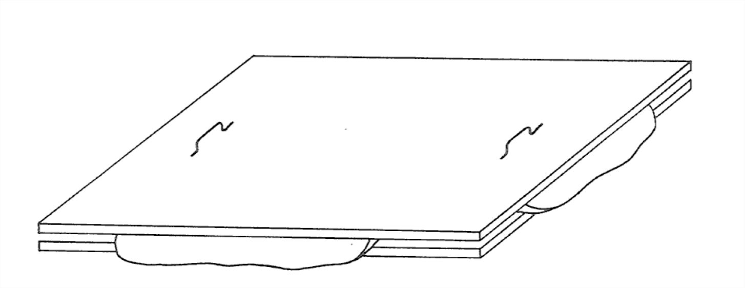
The viscosity of a fluid, usually denoted by μ, is a measure of the resistance of the fluid to deformation. Here’s a great kitchen experiment to introduce you to the concept of viscosity. Obtain two big sheets of plate glass, about the size of home window sashes. You will have to attach a couple of handles to the top surface of one of them, perhaps with suction cups of some kind. Lay one of them flat on your kitchen table or counter and slather it with a “thick” (read “viscous”) liquid, like honey, molasses, corn syrup, or motor oil (your choice). Right away, before the liquid starts to ooze off the glass, place the other piece of plate glass, the one with the handles, on top of the surface of the liquid (Figure 1-40). Be sure there are no trapped air bubbles.

Figure 1-40. Shearing a viscous fluid between two parallel plates

Now grip the handles and shift the upper plate horizontally at constant speed parallel to the lower plate, being careful to maintain constant spacing between the two plates. You will easily sense that the greater the relative speed of the plates, the greater the force needed to maintain the shearing of the fluid. The viscosity is just the coefficient associated with the ratio between the rate of shearing and the force (measured per unit area in the planes of shear) that resists the shearing:

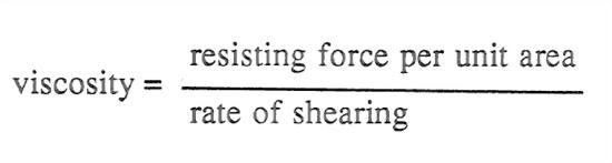
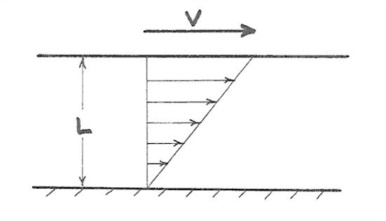
Here, the rate of shearing is measured by the speed of the upper plate relative to the stationary lower plate, divided by the spacing between the plates (Figure 1-41). For most common fluids, air and water included, this ratio is the same whatever the rate of shearing; such fluids are called Newtonian fluids.

Figure 1-41. Cross-section view through the kitchen-table-top experiment on shearing of a viscous fluid, showing the spacing L of the plates and the speed V of the upper plate relative to the lower plate. Also shown is the distribution of local fluid speed you would measure along a line between the two plates.

One more fluid property, the specific weight (in other words, weight per unit volume), usually denoted by , is important when the fluid is in a gravitational field, as on the earth's surface. The specific weight is the weight of the fluid per unit volume of fluid. It’s not the same as the density of the fluid, which is the mass per unit volume. For us earthbound beings, the ratio of the density to the specific weight is almost exactly constant, because the two are related by virtue of the acceleration due to gravity, g: = g. You can “uncouple” the density and the specific weight only by taking a trip in a space ship to another planet!

Now I want you to concentrate on what the fluid dynamicists call an open-channel flow. As the term implies, it’s just a flow in some kind of channel that’sopentotheairabove,ratherthanbeingenclosedwithinapipeorconduitas in your home plumbing system. To study open-channel flow you can play in the gutter after a brief heavy rainstorm, or park yourself next to a stream or river, or nail a channel together in your back yard and supply it by means of a hose. Such examples of channel flows, although rather different in scale and geometry, share most of their essential features.

Incidental but important note: It turns out that these open-channel flows differ from their pipe-flow cousins only in the presence of the so-called “free surface”, not in their essential behavior. Most of the flows we will touch upon in this course are open-channel flows, but when we deal with groundwater flow, you’ll see that pipe flow is the closer analogy.

There’s a wealth of variables you can use to describe the flow. Some are more concrete and easy to understand than others. On the one hand, you can think about the velocity of the flow, and on the other hand, you can think about the force per unit area the flow exerts on its boundary.

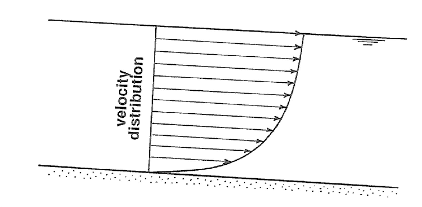
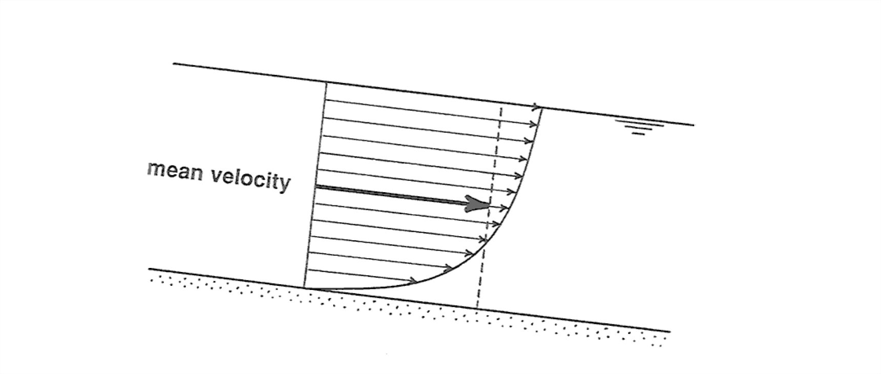
With regard to velocity, if you occupied any point in the flow that’s fixed relative to the boundaries and used a magic little velocity meter to measure the local fluid velocity, you would get some stable local time-average velocity if you continued your measurement for a fairly long time. This time-average local velocity varies continuously from point to point all over the cross section of the flow (Figure 1-42); more on what that distribution of local velocity looks like presently.

Figure 1-42. Time-average local velocity varies continuously from point to point all over the cross section of the flow

You can take the average of all the local velocities all over the flow cross section to get a mean flow velocity U (Figure 1-43). In real rivers this is how it’s actually done, but in laboratory channels, where it's easy to know the water discharge (the volume rate of flow), you can use the relationship Q = UA, where Q is the discharge and A is the area of the flow cross section, to find U.

Figure 1-43. Averaging all the local velocities all over the flow cross section to obtain the cross-section mean flow velocity

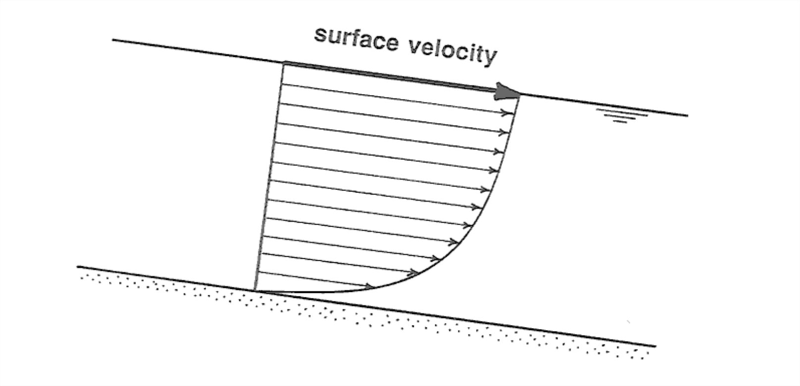
You could also measure the surface velocity Us along the centerline

of the flow (Figure 1-44). This is greater than the mean velocity, by a factor of something like 1.2 or 1.3; it's related to U in a rather complex way that needn't concern us here. Incidentally, unless the channel is very wide compared with the depth of flow the position of maximum velocity on the cross section lies a little below the surface.

Figure 1-44. The surface velocity, shown along with the velocity distribution in the interior of the flow.

The average force per unit area the flow exerts on its boundary, called the boundary shear stress, denoted by τo (read “tau sub zero” or “tau

naught”) is a little trickier to deal with than velocity, and is less concrete to visualize, but it’s important for the obvious reason that it’s what exerts forces on the sediment particles on the bed of a stream or river or on the surface of a sand dune under the wind.

Let me backtrack a little to point out something about the flow near the boundary that will probably seem very counterintuitive to you, but stands as a firmly established fact of observation: fluid in direct contact with a solid boundary has exactly the same velocity as that solid boundary. That’s called the no-slip condition. In the context of our open-channel flow, it means that the water right at the bed has zero velocity! But of course there is an increase in velocity upward from the bed, so all the water above the bed, no matter how small a distance above, generally has a nonzero velocity.

The reason I have brought in the no-slip condition here is this: the origin of shear stresses in fluids is just the existence of shearing itself. If that doesn’t make sense to you at first thought, go back to your sticky, messy kitchen- table-top experiment on shearing of a viscous fluid. The stronger the shearing, the greater the shear stress that’s generated, other things being equal. And foremost among those other things is the viscosity, introduced earlier.

So, back to the boundary shear stress τo. It’s true that if you could get right down close to any point on the channel bottom, you could (with the right instrument, which doesn’t actually exist!) measure a local shearing force per unit area the flow exerts on the solid boundary. That fits the term “boundary shear stress” well, but it’s not what's conventionally meant by the boundary shear stress. What you have to do is take a spatial average of the local shear stress (that is, the average of a large number of “point values” of the local shear stress) over an area large enough to include a large number of representative “roughness elements” (sand grains, or boulders, or even larger protuberances, whatever “non-planarities” happen to be present on the channel bottom).

1.6.3 More on Forces Exerted by Moving Fluids

So far you have learned that a fluid moving past a solid body exerts frictional (“viscous”) forces on the surface of the body. These are friction forces in the true sense of the term, even though the detailed nature of the force is not quite the same as the friction between a sliding brick and surface upon which it’s sliding. Aerodynamicists have developed a very expressive term for such frictional forces: skin friction (by reference to the “skin” of an airplane wing). But there’s another important kind of force exerted by moving fluids: pressure forces. These are forces exerted by the flow on what might be called blunt bodies or bluff bodies: those that present a “frontal surface” to the oncoming flow (Figure 1-45).

Figure 1-45. Flow around a blunt body.

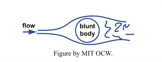
It will probably seem obvious to you that the fluid pressure (by pressure I mean force per unit area directed normal to a surface) on the upstream side of a blunt body is greater on the upstream side than the downstream side. What is much less obvious, but nonetheless true, is that, in absolute terms, the pressure on the front is greater than the “free-stream pressure” (the pressure in the fluid at some point far away from the body) but the pressure on the back is less than the free-stream pressure. It would take a lot more background work than we have time for to satisfy you that that’s true; you will have to take my word for it.

If you are inclined to doubt the foregoing statement, here’s a home experiment which (in contrast to many of my proposed home experiments) would actually be easy to do. All you need is a barometer, of the kind they now peddle as part of “home weather stations”. You would need a windy day for this experiment, and a single-family home. Close all of the doors and windows tightly, so there’s no throughgoing wind in the house. Stand next to the upwind side of your house and read the barometer. Now go around to the downwind side of the house and take a reading there too. You would find, of course, that the local atmospheric pressure on the downwind side is noticeably less than on the upwind side. That’s the real origin of the wind force that tends to blow your house down. But now walk far away from your house and take a barometer reading in an open and unobstructed area (you are now in that “free stream” I mentioned earlier). That reading will lie between the first two—showing that the local atmospheric pressure on the downwind side of the house is indeed lower than the free-stream pressure!

The pressure difference, fore and aft, means that the fluid pressure is exerting a net force in the downstream or downwind direction on the bluff body; it’s just a matter of adding a larger downstream-directed force (call that the positive direction) and a smaller upstream-directed force (call that the negative direction); the result is a positive downstream force. This kind of force is very expressively called pressure drag or form drag.

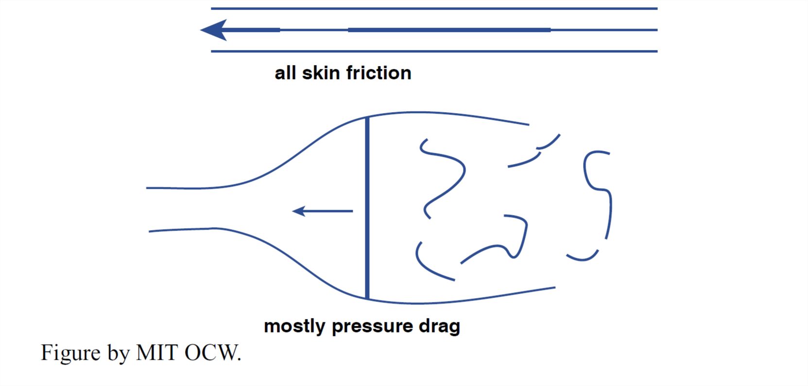
Except for very small-scale flows and very slow velocities, the pressure drag is likely to be much larger than the skin friction. Does that make sense to you? Probably not, because I don’t think it’s “intuitively obvious”. If not, then here’s still another experiment, another one that would be easy in real life, that you can do for yourself to demonstrate the truth of that proposition. It’s probably the simplest experiment I’ll propose all semester: all you would need is a pizza pan and a swimming pool! Stand in water up to your chest, and move the pan through the water in the direction parallel to itself. It slips easily through the water, right? Now turn it so that the surface of the pan is normal to the direction of movement. It takes a far greater force on your part to move the pan through the water in that orientation than before. That’s because the front-to-back pressure difference adds up to a much greater force than just the frictional forces on the two surfaces of the pan when it’s moved parallel to itself (Figure 1-46).

Figure 1-46. Skin friction and pressure drag on a pizza pan moved through still water.

1.6.4 Why Do Fluids Move?

The movement of fluids is part of the experience of our daily lives. But it’s valuable to think for a moment about why fluids move. According to Newton’s first law of motion, a body moves in a state of uniform motion (changing neither speed nor direction) unless it is acted upon by some force. Moving fluids are always acted upon by friction, so they come to rest unless some other force is available to offset the friction and keep them in motion.

Two important kinds of forces drive fluid motions:

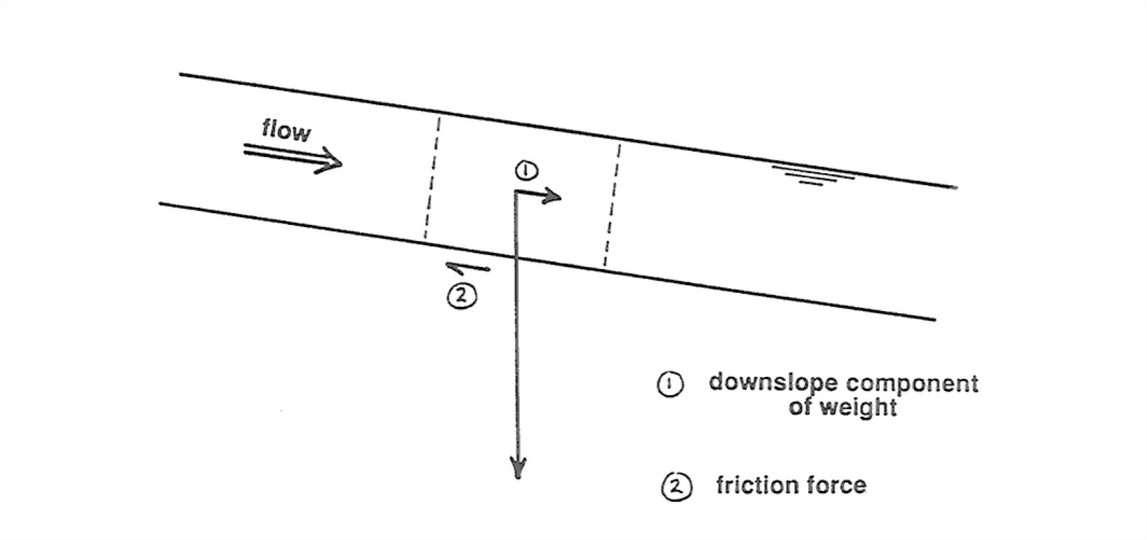
• The force of gravity. In a flow down a sloping channel, the weight of an element of fluid has a downslope component (Figure 1-47). This downslope component of fluid weight counterbalances the frictional resistance exerted on the fluid by the bottom boundary.

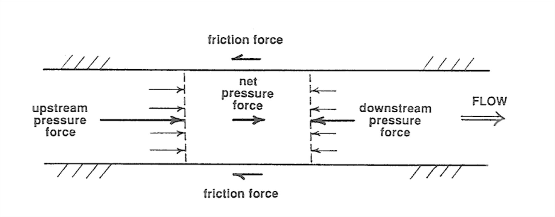
• Pressure gradients. In a flow in a horizontal pipe or conduit, the fluid moves only if there is a downstream decrease in fluid pressure. To see why this causes the fluid to move, look at an element of fluid in the pipe (Figure 1-48). If there is a downstream pressure gradient (that is, the pressure decreases in the downstream direction), then the force on the upstream face of the element is greater than the force on the downstream face. The difference in forces on the upstream and downstream faces is a force directed downstream. This downstream force counterbalances the frictional resistance exerted on the fluid by the walls of the pipe.

Figure 1-47. In a flow in a horizontal pipe or conduit, the fluid moves only if there is a downstream decrease in fluid pressure.

In a general fluid flow, both of these kinds of forces (downslope gravity components and downstream pressure gradients) can be present at the same time, and the fluid moves under their combined effect.

1.6.5 Channel Flows

Now let’s think about what the flow really looks like in a large channel flow like a river. The basic picture is as shown in Figure 1-48: there’s a balance between the downchannel pull of gravity on the fluid, which acts throughout the flow, and the resistance force the bed and banks exert on the flowing fluid, which is equal and opposite to the boundary shear stress we discussed above. A natural consequence of the action of these two different forces—gravity acting throughout the fluid and the resistance force acting only at the boundary—is that the velocity increases upward in the flow, from zero at the boundary, by the no-slip condition, to a maximum at or near the surface.

Figure 1-48. In a flow down a sloping channel, the weight of an element of fluid has a downslope component that’s balanced by the friction force the boundary exerts on the flow.

That’s only the crudest first-order picture, though: the question comes naturally to mind: what are the details of the distribution of time-average local flow velocity over the entire cross section of the flow? That’s much too intricate a question for us to pursue here, so I will just hit the high points.

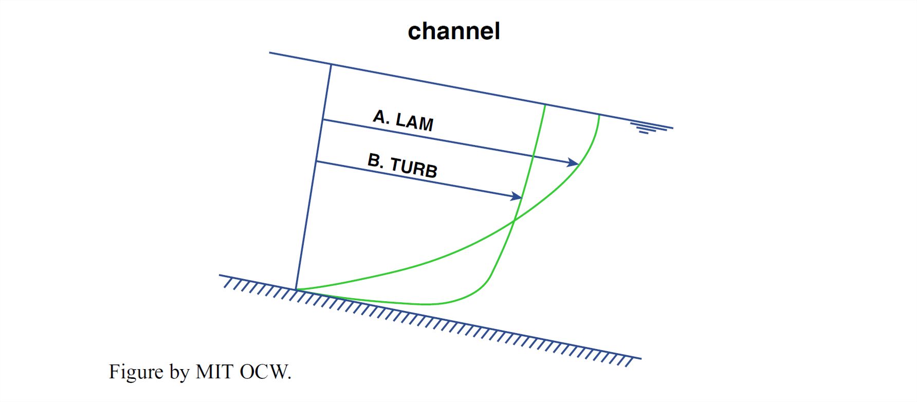
It’s simplest to think about a river with a large width-to-depth ratio, which is usually the case. Then we can forget about the effect of the banks. A straightforward application of Newton’s laws, which I’ll have to skip over here, shows that the distribution of velocity should be parabolic (Figure 1-49A), with the vertex of one limb of a parabola located at the surface. (If you are inclined to pursue this matter further, look me up, and I will set the problem for you to work on.)

But if you went out and measured the local time-average velocity at a series of points along a vertical from the surface down to the bottom, you would find the actual distribution to be far from parabolic: the distribution would be much more uniform over most of the flow depth, and the necessary decrease to zero at the boundary would be in a very thin zone right next to the boundary. The distribution would closely approximate a logarithmic distribution (Figure 1-49B). The reason why the distribution is close to being logarithmic is beyond the scope of this course, but you can readily understand why the qualitative shape of the curve is the way it is, with a much smaller velocity change throughout most of the flow depth but a sharply greater velocity change right near the bottom. To see why, however, we have to do a little more preparatory work; read on.

Figure 1-49. Laminar and turbulent velocity profiles in open-channel flow.

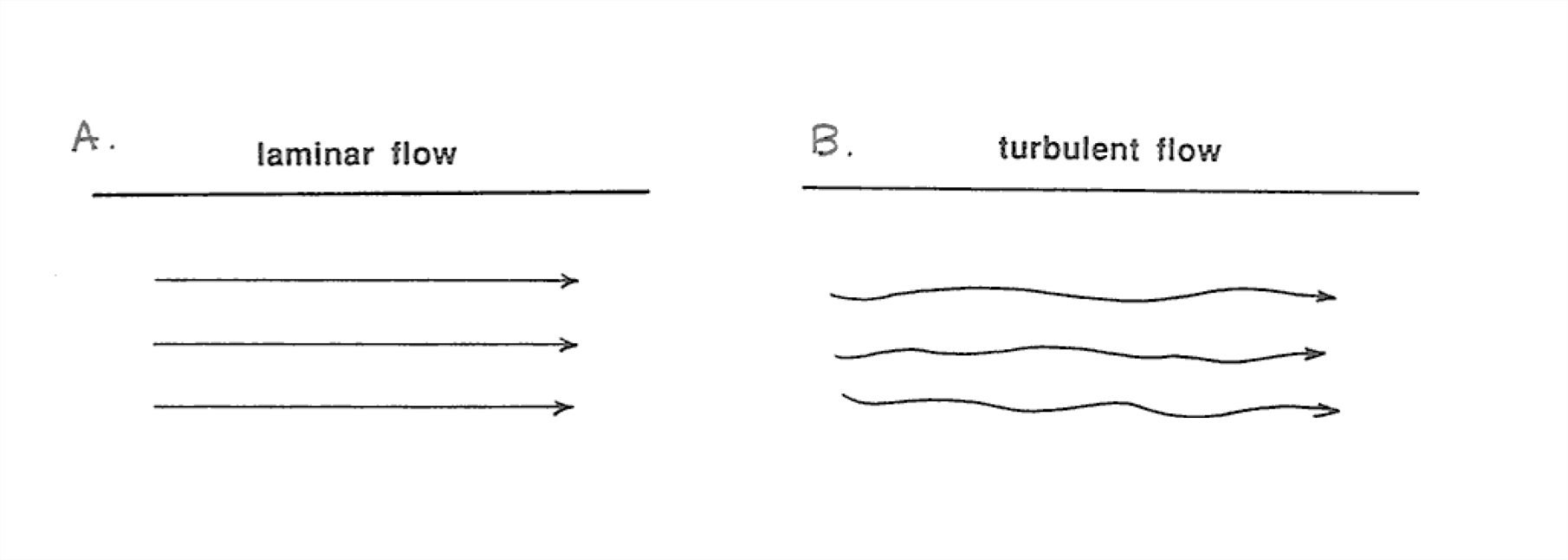
This difference in velocity profiles has to do with the difference between laminar flow and turbulent flow, which I am sure you have all heard about one way or another. Channel flows that are very shallow and/or very slow- flowing (like sheet flow or overland flow on the land surface during and after a rain) are characterized by the regular and locally rectilinear flow trajectories of laminar flow (Figure 1-50A), whereas channel flows that are deeper and/or faster- moving (almost all channelized flows fall into this category) show the irregularly sinuous flow trajectories characteristic of turbulent flow (Figure 1-50B).

Figure 1-50. Paths of fluid elements in A) laminar flow and B) turbulent flow.

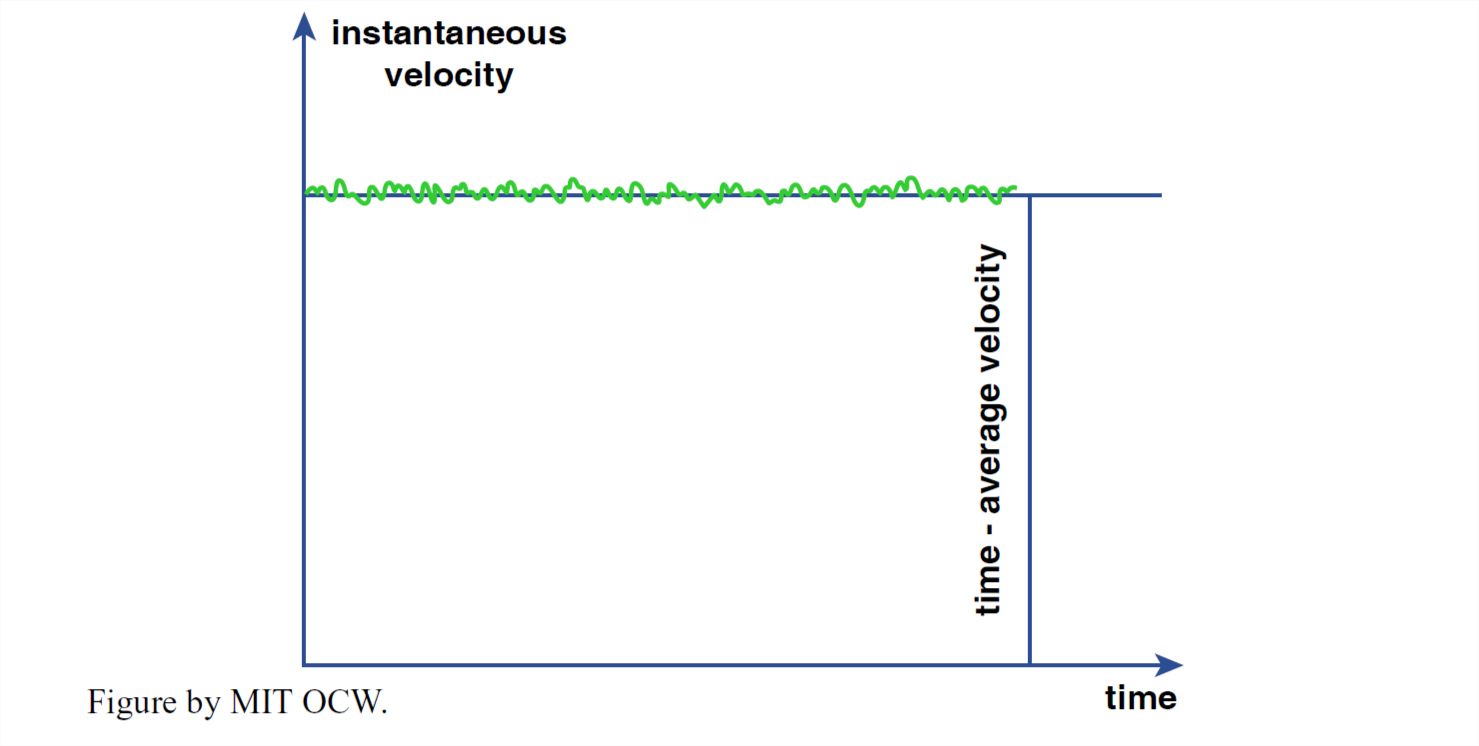
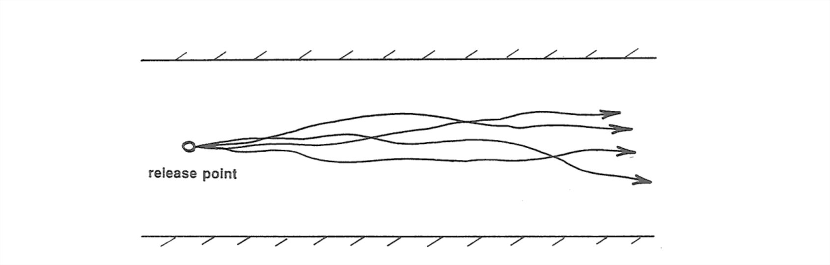
Turbulence isn’t easy to describe, but because it’s such an important aspect of fluid flows on the earth’s surface I’ll attempt to give you a qualitative picture of what turbulence is like, with channel flow as the example. One way of studying turbulence is to make a continuous measurement of velocity as a function of time at a fixed point in the flow. You would obtain a record that looks something like the graph shown in Figure 1-51: velocity fluctuations with a range of magnitudes and time scales would be present around the time-average velocity. Another way of seeing the turbulence is to release small neutrally buoyant markers from some fixed point in the flow and watch them move downstream (Figure 1- 52). The trajectories would be irregularly sinuous, with angles of deviation from the downstream direction amounting to no more than several degrees. Each trajectory would be different in detail from all of the others.

Figure 1-51. Typical record of a continuous measurement of velocity as a function

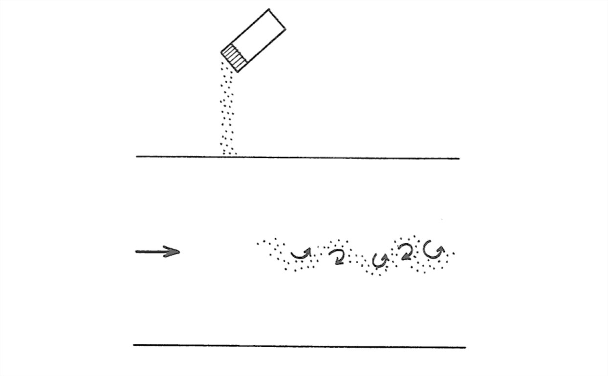
The best way to see the turbulence, however, is to sprinkle the flow with magic powder that allows you to see the turbulent eddies (Figure 1-53). You would see rotating swirls of fluid that grade continuously into one another and that change their shape continuously with time. Individual eddies retain their identity for a certain period of time (larger eddies live longer than smaller eddies). but any given eddy eventually becomes unrecognizable and is replaced with newly developed swirls. The flowing surface of a river carrying fine sediment in suspension shows eddies moving up to the water surface to spread out and flatten themselves. You might also watch smoke or steam issuing from a smokestack to see the production and decay of eddies as the plume of hot stack gases rises through the still ambient air.

Figure 1-52. Trajectories of small neutrally buoyant marker particles released from some fixed point in a turbulent channel flow.

Figure 1-53. Sprinkling the flow with magic powder that allows you to see the eddies.

The maximum vertical scale of eddies in the flow is not much smaller than the depth of the flow, and the maximum cross-flow scale is even larger. There’s a continuous range of sizes down to very small eddies, of the order of fractions of a millimeter. The smaller eddies are superimposed on the larger eddies. As the large eddies sweep along the boundary they cause periods of stronger flow and weaker flow. When you’re standing on a broad plain or on the deck of a ship at sea, the wind gusts you feel are a manifestation of these large eddies affecting the flow boundary. Have you ever watched a broad field of tall grass or grain in a strong wind from a point high above? You would see a striking pattern of wind gusts moving along in the direction of the wind as they sway the grass.

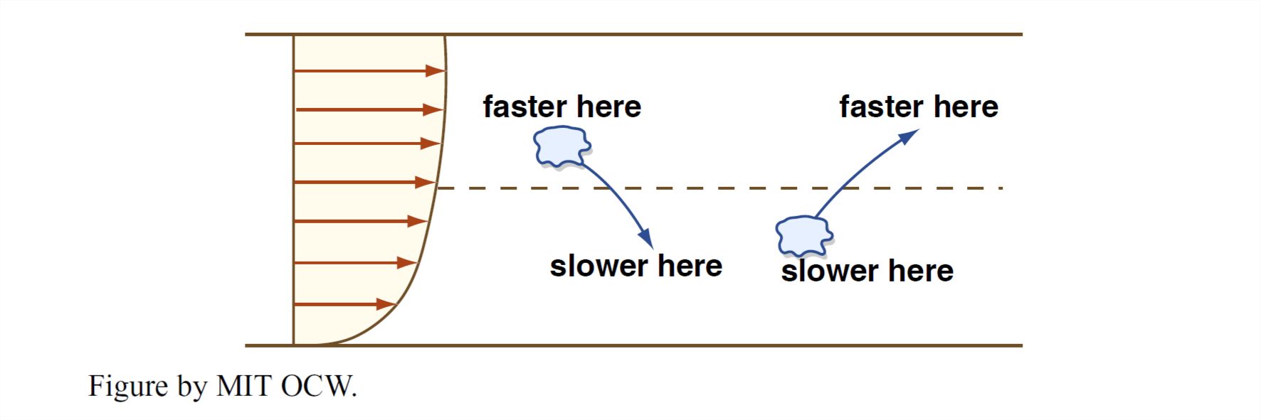
Returning now to the important qualitative difference between laminar and turbulent velocity distributions, in turbulent flow the velocity distribution is much more uniform over most of the thickness of the flow but changes much more sharply very close to the boundary. It’s easy to understand why this is so (Figure 1-54). In turbulent flow, over most of the flow depth the lateral motions of eddies tend to even out the differences in time-average velocity from layer to layer. Here’s how this works (keep in mind the overall average upward increase in flow speed): upward-moving eddies tend to arrive at their new surroundings with a speed slower than their new surroundings, so they tend to slow those new surroundings down. Conversely, downward-moving eddies tend to arrive in their new surroundings with a speed faster than their new surroundings, to they tend to speed those new surroundings up.

Figure 1-54. Why the velocity profile in turbulent flow is blunter over most of the profile than in laminar flow.

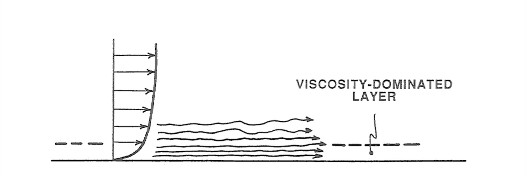
As we move closer and closer to the boundary, however, the fluid motions perpendicular to the boundary are more and more restricted—because remember that right at the boundary the fluid velocity must match that of the boundary, so there can be no component of velocity normal to the boundary there. In a thin layer next to the boundary, therefore, the turbulence can’t even out the differences in velocity from layer to layer, so the gradient of velocity is very steep. This layer next to the boundary, where viscous shearing is more important than turbulence, could be called the viscosity-dominated layer (Figure 1-55). Its thickness is typically a very small percentage of the flow depth, no more than millimeters to at most a few centimeters. The next time you’re sitting in a window seat in the jetliner, look out at the surface of the wing and think about that viscosity-dominated layer. The air speed, relative to the surface of the wing, decreases from its free-stream value of several hundred miles per hour to zero over a thickness of centimeters, and the viscosity-dominated layer is a small fraction of a millimeter. Incidentally, the cross-section shape of the wing (the “airfoil”) is designed to minimize pressure drag, so in this case the body (the wing) is not really a blunt body at all! The reason the plane stays in the air is that the local air pressure on the upper surface of the wind is less than on the lower surface, but the aerodynamic reason for this would require a lot more work on your part.

Figure 1-55. The viscosity-dominated layer at the base of a turbulent channel flow.

1.6.6 Oscillatory Flows

Everything in the preceding sections is relevant to unidirectional flow: a current that moves in one direction only, with velocity either unchanging with time (steady flow) or changing somehow with time (unsteady flow). Also important in the transport of sediments is oscillatory flow: a current that reverses its direction periodically with time. The approach in this section will be somewhat different from the approach in the preceding sections: I’ll concentrate more on the origin and description of oscillatory flows than on their dynamics.

Except for reversing tidal currents, which technically are oscillatory flows with very long oscillation periods but which are better considered as reversing unidirectional flows, almost all of the important oscillatory flows in nature are caused by surface gravity waves which propagate on the surfaces of oceans and large lakes. Such waves are called surface waves because they are associated with the water surface, and they’re called gravity waves because the dominant force involved in their propagation (the force which attempts to restore the deformed water surface to a planar condition) is the force of gravity.

The generation of wind waves is a complex process, even now not fully understood, that involves both the shear stress of the moving air on the water surface and on the unequal distribution of air pressure over the windward and leeward sides of geometrical irregularities on the water surface. I’ll note here only that the size of the waves depends on three factors: the speed of the wind, the duration of time the wind acts on the water surface, and the downwind distance (called the fetch) over which the wind acts on the water surface.

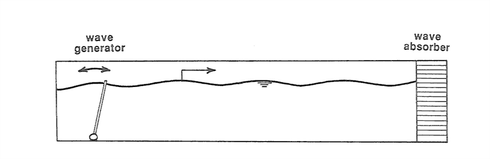
The best way to obtain an idea of the basic nature of the water motions produced by surface gravity waves is to watch the propagation of a single train of waves in a wave tank (Figure 1-56). You can imagine building a long tank with rectangular cross section, perhaps several meters long, open at the top. Put a wave generator at one end. A board hinged to the bottom of the tank can be rocked or oscillated back and forth to produce a train of waves. It’s best to install some porous material at the other end of the tank to absorb the waves, so that they're not reflected to interfere with the propagating wave train.

Figure 1-56. Making waves in a backyard wave tank.

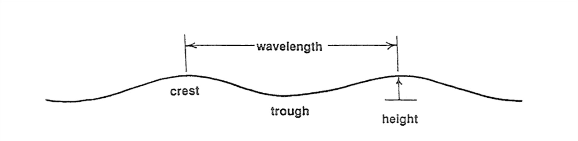
Here are some terms used to describe the waves in a simple train of waves (Figure 1-57). The crest of the wave is the highest point on the wave profile, and the trough is the lowest point on the wave profile. The period of the wave is the time needed for one complete wave form to pass a point that is fixed relative to the bottom of the tank. Surface gravity waves in natural environments have periods that range from less than a second to almost twenty seconds. The wavelength of the waves is the distance from crest to crest or from trough to trough. The height of the waves is the vertical distance from trough to crest. The heights of large waves generated by major storms are commonly in the range of five to fifteen seconds

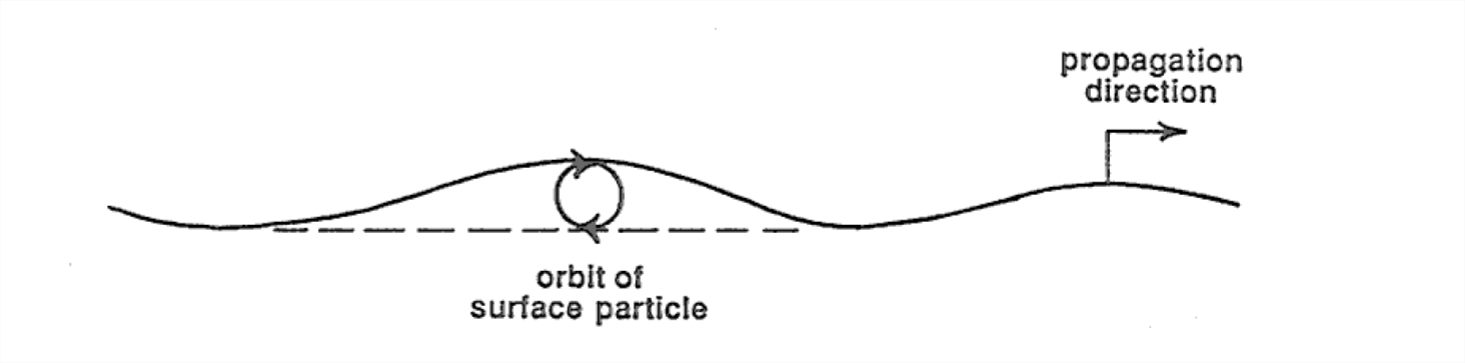
If you place a floating cork on the water surface and watch its motion through the wall of the tank as the waves pass by, you see that the cork travels in an almost perfectly circular orbit, making one circle during the passage of each wave (Figure 1-58). The sense of motion is such that the cork moves in the direction of wave propagation while the crest of the wave is passing, and opposite to the direction of wave propagation while the trough of the wave is passing.

Figure 1-57. Some terms used to describe the waves in a simple train of waves.

Figure 1-58. The circular orbit of a particle floating on the water surface as a wave passes.

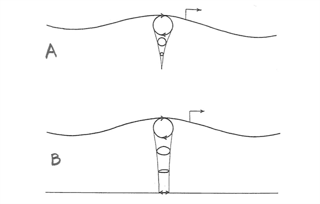
The water below the surface also moves as the waves pass, but the size of the orbits of the water particles decreases very rapidly with depth below the surface (Figure 1-59). The size of the orbits at a depth equal to half a wavelength is only about ten percent of the size of the orbits at the surface, and the size of the orbits at a depth equal to one full wavelength is negligible. Such waves are called deep-water waves. If the wavelength of the waves is much greater than the water depth, however, the size of the orbits is still appreciable at the bottom (Figure 1- 59). Such waves are called shallow-water waves, and they are common during storms. Downward from the surface the orbits become flattened into ellipses with greater and greater eccentricity, until at the very bottom the orbits are back-and- forth straight lines. This should make sense to you, because at the bottom there can be no fluid motion perpendicular to the bottom—if the slight flow into and out of the porous sediment is ignored.

Figure 1-59. A) Decrease in orbital diameter with depth beneath a deep-water wave. B) Decrease in orbital diameter beneath a shallow-water wave.

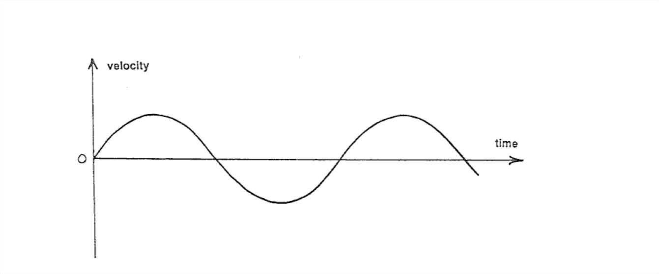
Now examine more closely the nature of the oscillatory water motion at the bottom. If you measured the fluid velocity near the bottom as a function of time at a point which is fixed relative to the bottom, you would obtain a record that looks like the graph in Figure 1-60: the velocity varies sinusoidally with time. The nature of the motion can be characterized by its period T, or by the maximum velocity U_m that is attained during one oscillation cycle (this happens when the water is at the central point of its oscillation path), or by the distance d_o moved by a water particle during one full oscillation (this is called the orbital diameter).

It’s part of the physical nature of waves that different trains of surface gravity waves can be superimposed on each other in such a way that the water-surface height and water motion at a given point is the sum of contributions from each superimposed wave train. You might know from watching storms at sea or on large lakes that the sea state produced by a strong wind is complicated, because it’s a superposition of a large number of separate trains of waves with slightly different periods, propagation directions, and heights. Also, when the wind direction changes as a storm passes, the waves adjust their direction of propagation in response. In such cases, the pattern of water movement at the bottom is no longer a simple back-and-forth movement. Even the relatively simple case of two regular trains of waves moving in different directions, the water movement on the bottom can be surprisingly complicated, to say nothing of the really complicated wave conditions produced during storms.

Figure 1-60. Fluid velocity near the bottom as a function of time at a point that’s fixed relative to the bottom, as a shallow-water wave passes by overhead.

1.6.7 The Wind

The large-scale structure of the lower part of the atmosphere is obviously much different from that of even the largest river. The most obvious difference is the absence of a free surface in the atmosphere. An equally important difference has to do with the much larger scale of wind systems. This is important because the Earth’s rotation plays a dominant role in determining wind direction (but this is not the course in which to pursue that very counterintuitive but fascinating matter) but is a minor aspect of even the largest of rivers. A third important difference is related to the easy compressibility of air, in contrast to the incompressibility of water. This means that the thermodynamics of compressibility plays an essential role in the behavior of the atmosphere.

Despite these far-reaching differences, it’s fortunate for us as earthbound creatures that the structure of the wind in the near-surface layer, up to hundreds or even a few thousands of meters above the surface, is usually not greatly different from that of large-scale channel flows, in terms of such things as velocity distribution, turbulence structure, and boundary forces. Most of what I said in earlier sections of this chapter for channel flows of water is applicable to the wind. This is especially true of eolian sand transport and the shaping of sand dunes.

You might complain that the wind is so much more gusty than the ordinarily turbulent flow of rivers. I would counter that by saying that your conception of the gustiness of the wind is shaped by observations made for the most part down in among large and very irregularly shaped and irregularly distributed roughness elements like trees, hills, and buildings. To the extent that things like that occupy river bottoms (hills are certainly there, and we’ll have to deal with them as a really important part of this course), and you sensed turbulence down at their level, flow in rivers would seem pretty “gusty” too. (There will be more on that later, when we talk about flow over subaqueous bed forms.) If you have ever experienced a strong wind at sea, you know that the wind unimpeded by large roughness elements is surprisingly steady.