19: Climate Change (Exercises)

Last updated
Save as PDF

Page ID: 2059

\( \newcommand{\vecs}[1]{\overset { \scriptstyle \rightharpoonup} {\mathbf{#1}} } \) \( \newcommand{\vecd}[1]{\overset{-\!-\!\rightharpoonup}{\vphantom{a}\smash {#1}}} \)\(\newcommand{\id}{\mathrm{id}}\) \( \newcommand{\Span}{\mathrm{span}}\) \( \newcommand{\kernel}{\mathrm{null}\,}\) \( \newcommand{\range}{\mathrm{range}\,}\) \( \newcommand{\RealPart}{\mathrm{Re}}\) \( \newcommand{\ImaginaryPart}{\mathrm{Im}}\) \( \newcommand{\Argument}{\mathrm{Arg}}\) \( \newcommand{\norm}[1]{\| #1 \|}\) \( \newcommand{\inner}[2]{\langle #1, #2 \rangle}\) \( \newcommand{\Span}{\mathrm{span}}\) \(\newcommand{\id}{\mathrm{id}}\) \( \newcommand{\Span}{\mathrm{span}}\) \( \newcommand{\kernel}{\mathrm{null}\,}\) \( \newcommand{\range}{\mathrm{range}\,}\) \( \newcommand{\RealPart}{\mathrm{Re}}\) \( \newcommand{\ImaginaryPart}{\mathrm{Im}}\) \( \newcommand{\Argument}{\mathrm{Arg}}\) \( \newcommand{\norm}[1]{\| #1 \|}\) \( \newcommand{\inner}[2]{\langle #1, #2 \rangle}\) \( \newcommand{\Span}{\mathrm{span}}\)\(\newcommand{\AA}{\unicode[.8,0]{x212B}}\)

Q19.1 Climate Change at the K-Pg Boundary

The short-term climate impact was significant cooling because the dust (and sulphate aerosols) would have blocked incoming sunlight. This effect may have lasted for several years, but its intensity would have decreased over time.

The longer-term impact would have been warming caused by the greenhouse effect of the carbon dioxide.

Q19.2 Albedo Implications of Forest Harvesting

Clear-cutting (or any logging activity) leads to a net increase in albedo, so the albedo-only impact is cooling.

Q19.3 What Does Radiative Forcing Tell Us?

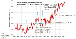
Using the ΔT = ΔF * 0.8 equation the expected temperatures for 2011, 1980 and 1950 compared with the estimated 13.4 C in 1750 should be:

2011 vs 1750 ΔT = 0.8 * 2.29 = 1.8°C (13.4 + 1.8 = 15.2)

1980 vs 1750 ΔT = 0.8 * 1.25 = 1.0°C (13.4 + 1.0 = 14.4)

1950 vs 1750 ΔT = 0.8 * 0.57 = 0.5°C (13.4 + 0.5 = 13.9)

[SE from data at NASA at: data.giss.nasa.gov/gistemp/ta...B.Ts+dSST.txt]

Based on this reasoning the estimated temperature for 1950 is13.9˚ C (which is close to the actual of 14.0 ˚ C), while that for 1980 is 14.4˚ C, which is well above the actual of 14.2˚ C. It’s also clear that we didn’t reach 15.2˚ C by 2011, because even in the hottest year so far (2015) the global average temperature was only 14.8˚ C.

So while the ΔT = ΔF * 0.8 equation is useful, it appears to overestimate the temperature, probably because it takes some time (years to decades) for the climate to catch up to the forcing.

Q19.4 Rainfall and ENSO

Describe the relationship between ENSO and precipitation in B.C.’s southern interior.

As shown on the diagram below, there are some examples where a strong ENSO signal corresponds with very strong precipitation in the interior (and on the coast as well). The two strongest El Niños (1983 and 1998) shown correspond with the highest recorded precipitation levels in Penticton. Some other strong El Niños (1958 and 1973) are associated with strong precipitation within 6 months of the ENSO peak, but others show a negative correlation between ENSO and rainfall (marked with “?”).

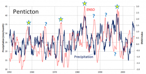
[SE using climate data from Environment Canada, and ENSO data from: www.esrl.noaa.gov/psd/enso/mei/table.html]

Q19.5 How Can You Reduce Your Impact on the Climate?

Responses will vary