

14.3: Principle of Limiting Factors
- Page ID
- 42729

\( \newcommand{\vecs}[1]{\overset { \scriptstyle \rightharpoonup} {\mathbf{#1}} } \)
\( \newcommand{\vecd}[1]{\overset{-\!-\!\rightharpoonup}{\vphantom{a}\smash {#1}}} \)
\( \newcommand{\dsum}{\displaystyle\sum\limits} \)
\( \newcommand{\dint}{\displaystyle\int\limits} \)
\( \newcommand{\dlim}{\displaystyle\lim\limits} \)
\( \newcommand{\id}{\mathrm{id}}\) \( \newcommand{\Span}{\mathrm{span}}\)
( \newcommand{\kernel}{\mathrm{null}\,}\) \( \newcommand{\range}{\mathrm{range}\,}\)
\( \newcommand{\RealPart}{\mathrm{Re}}\) \( \newcommand{\ImaginaryPart}{\mathrm{Im}}\)
\( \newcommand{\Argument}{\mathrm{Arg}}\) \( \newcommand{\norm}[1]{\| #1 \|}\)
\( \newcommand{\inner}[2]{\langle #1, #2 \rangle}\)
\( \newcommand{\Span}{\mathrm{span}}\)
\( \newcommand{\id}{\mathrm{id}}\)
\( \newcommand{\Span}{\mathrm{span}}\)
\( \newcommand{\kernel}{\mathrm{null}\,}\)
\( \newcommand{\range}{\mathrm{range}\,}\)
\( \newcommand{\RealPart}{\mathrm{Re}}\)
\( \newcommand{\ImaginaryPart}{\mathrm{Im}}\)
\( \newcommand{\Argument}{\mathrm{Arg}}\)
\( \newcommand{\norm}[1]{\| #1 \|}\)
\( \newcommand{\inner}[2]{\langle #1, #2 \rangle}\)
\( \newcommand{\Span}{\mathrm{span}}\) \( \newcommand{\AA}{\unicode[.8,0]{x212B}}\)
\( \newcommand{\vectorA}[1]{\vec{#1}} % arrow\)
\( \newcommand{\vectorAt}[1]{\vec{\text{#1}}} % arrow\)
\( \newcommand{\vectorB}[1]{\overset { \scriptstyle \rightharpoonup} {\mathbf{#1}} } \)
\( \newcommand{\vectorC}[1]{\textbf{#1}} \)
\( \newcommand{\vectorD}[1]{\overrightarrow{#1}} \)
\( \newcommand{\vectorDt}[1]{\overrightarrow{\text{#1}}} \)
\( \newcommand{\vectE}[1]{\overset{-\!-\!\rightharpoonup}{\vphantom{a}\smash{\mathbf {#1}}}} \)
\( \newcommand{\vecs}[1]{\overset { \scriptstyle \rightharpoonup} {\mathbf{#1}} } \)
\(\newcommand{\longvect}{\overrightarrow}\)
\( \newcommand{\vecd}[1]{\overset{-\!-\!\rightharpoonup}{\vphantom{a}\smash {#1}}} \)
\(\newcommand{\ket}[1]{\left| #1 \right>}\)
\(\newcommand{\bra}[1]{\left< #1 \right|}\)
\(\newcommand{\braket}[2]{\left< #1 \vphantom{#2} \right| \left. #2 \vphantom{#1} \right>}\)
\(\newcommand{\braopket}[3]{\left< #1 \vphantom{#2}\vphantom{#3} \right| #2 \vphantom{#1}\vphantom{#3} \left| #3 \vphantom{#1}\vphantom{#2} \right>}\)
\(\newcommand{\qmvec}[1]{\mathbf{\vec{#1}}}\)
\(\newcommand{\op}[1]{\hat{\mathbf{#1}}}\)
\(\newcommand{\expect}[1]{\langle #1 \rangle}\)
\(\newcommand{\dfn}[1]{\emph{\textbf{#1}}}\)
Plant hardiness zones and climate change
The plants and animals that succeed in occupying a particular niche are those that can easily adapt to the unique environmental conditions of a site. Each plant and animal in the community has a specific range of tolerance for particular environmental conditions. Climate factors are the most important influence over the successful establishment of plant and animal communities. Two climatic factors are important, sunlight and moisture.
Not only is the amount of sunlight available important but the duration and quality of light are important too. For instance, at high altitudes the intense ultra violet light may inhibit the growth of particular plants. The intensity of light affects photosynthesis and rate of primary productivity. The duration of sunlight affects the flowering of plants and the activity patterns of animals. The availability of water is important for the survival of most life forms. But plants require water for a number of life processes like germination, growth and reproduction too. The principle of limiting factors says that the maximum obtainable rate of photosynthesis is limited by whichever basic resource of plant growth is in least supply. The availability of energy and moisture varies geographically. At high latitudes the limiting factor is generally energy availability while in low latitudes moisture is the limiting factor to growth. The diagram below shows the relationship between potential evapotranspiration, a moisture index, climate and vegetation.
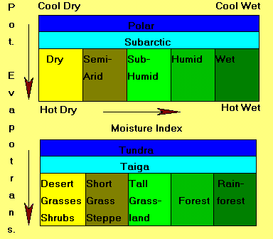
Figure \(\PageIndex{1}\) shows the relationship between climate and vegetation using two environmental variables: potential evapotranspiration (PE) and a moisture index (MI). Potential evapotranspiration serves as a proxy for temperature and energy availability, represented on the vertical axis, while the moisture index is shown on the horizontal axis, ranging from dry conditions on the left to wet conditions on the right.
Potential evapotranspiration is the optimal amount of water entering the atmosphere as a result of evaporation and plant transpiration when there is an unlimited amount of moisture. Because evaporation and transpiration depend on energy availability, potential evapotranspiration is a measure of energy input. High values of potential evapotranspiration relate to warm climates while low values to cool climates. The moisture index is a measure of moisture availability. High values of the moisture index means that plenty of water is available. Combining the two variables, potential evapotranspiration and moisture index we have a notion of what the climate is like in any part of the diagrams. For instance, high PE and large values of MI are indicative of warm and moist climates. Note that tundra and taiga (mostly conifers) are successfully established over a wide range of moisture conditions, from dry to moist, but always in cool environments. Other vegetation systems have more narrowly defined moisture and temperature requirements.
Plants of a particular region have adapted to the temperature and moisture conditions in which they live. Most gardeners are familiar with plant hardiness (growing) zone maps. The zones are based on the minimum temperature experienced and thus tolerated by different species of plants. There have been recent signs that these zones are starting to shift due to global warming.