10.4: Stream Gradation

The Davisian Cycle and Stream Development

The characteristics of a stream channel represents a balance between the amount of water flowing through it, the material the channel is located in, and the relief of the region in which the channel has formed. The famous physical geographer William Morris Davis proposed a theory of landscape development that describes a cycle of erosion which shapes the land surface. Though an over simplification of the true process, and one that is difficult to apply in many situations, it is nonetheless an interesting way of envisioning how a stream system forms and evolves.

Figure \(\PageIndex{1}\): Vertical cutting is typical of the early stages of stream system development which is evident in the image of Dynjandi, a series of waterfalls located in the Westfjords (Vestfirðir), Iceland.(CC BY-SA 4.0; By Diego Delso via Wikimedia Commons).

The Davisian Cycle 

Conceptually, the Davisian Cycle of erosion is based on the idea that landforms go through a sequence of orderly changes that range from an initially uplifted stage to a flat low relief stage also known as a peneplain. The model is based on structure of the rock types and their arrangement, the agents of erosion like rivers, wind, waves and ice acting on the landforms and the duration for which the agents of erosion act on the land. The cycle was divided into three main stages which are Youth, Maturity and Old Age. The model assumes that uplift occurs first after which their is a period where there is no further uplift also called tectonic quiescence during which the agents of erosion model and shape the landscape. 

Youthful stage is considered the beginning of the Davisian cycle where in a recently uplifted region stream system forms. Vertical erosion by rivers is the most prominent process when the river actively erodes downwards towards base level , the theoretical limit to which a stream can erode its channel. For streams entering the ocean, base level is sea level. For tributary streams, it is the elevation of the stream into which the tributary joins. During this early stage, rivers cut deep , narrow V-shaped valleys with features like water falls, rapids, gorges, narrow channels, and little flood plain area beside the stream. 

In the mature stage, vertical erosion slows down and lateral processes like valley widening become more important. Meanders become predominant as the drainage system becomes well integrated into the landscape. Rivers meander along broader valleys and form floodplains.  In this stage sharp ridges and valleys are common. In the early stage of maturity maximum relief is reached after which lateral erosion widens the valleys and lowers the divide leading to overall reduction in relief. 

Old age stage is the last stage in the Davisian cycle of erosion where there is a strong focus on deposition. In this stage vertical and lateral erosion slows down. Monadnocks, which are scattered isolated hills of resistant rocks, are found in this stage. As meandering channels wear away at interfluves, the surface is worn down to a plain of low relief called a peneplain. The landscape remains in its "old age" stage until uplift renews the cycle.

Even though Davisian Cycle was a very significant concept in geomorphology for providing a systematic way to understand landform development , it has been widely criticized for its assumptions like uplift is a single event followed by tectonic stability. Modern geomorphology favors the concept of dynamic equilibrium where uplift and erosion occur simultaneously. 

Modern Theories

Modern theories of landscape development suggests that stream system development achieves a dynamic equilibrium between the system and its environment. The equilibrium state is determined by the balance between inputs and outputs from the system. Over time, the channel achieves an equilibrium state between inputs (water) and outputs (sediment). Once equilibrium is achieved it remains in this state until a disturbance alters the inputs and outputs of the stream system.

The Graded Stream

In several cases throughout this book we have noted that natural open systems tend toward a state of equilibrium and stream systems are no different. Over a long period of time, the gradient of a stream adjusts so that the average load of sediment is balanced by that which it receives from surrounding slopes and in-flowing channels. For example, if sediment accumulates in stream, the bed of the channel is raised and the slope of the stream increases downstream of the deposit. Increasing the slope results in a higher stream velocity thus increasing the water's ability to move sediment. Eventually, a channel slope is reached that can carry away the accumulated sediment. Conversely, if sediment delivery to the stream is reduced, down cutting of the channel ensues. Channel erosion lowers the stream gradient until the material contributed to the stream is equal to that which is transported through it. Once a stream adjusts its gradient for the local environmental conditions is referred to as a graded stream.

 

Figure \(\PageIndex{2}\): Longitudinal Stream Profile. (CC BY-SA 4.0; Curated by Michael Ritter in The Physical Environment).

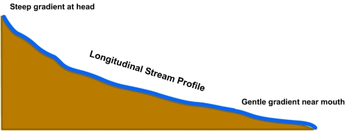
The longitudinal profile  as shown in Figure \(\PageIndex{2}\) is a depiction of the down slope gradient of a stream. The longitudinal profile of a stream can reveal if a stream has achieved a graded state, whether over a part or the entire stream. The curved profile of a graded stream exhibits a steeper slope upstream giving way to a gentle slope in the down valley direction. Initially stream profiles may be irregular with the stream gradient interrupted by knickpoints where waterfalls are found. Knickpoints as shown in Figure \(\PageIndex{3}\), are sharp local changes in the slope of a river's channel and represent a discontinuity in its longitudinal profile.  Knickpoints form where the stream flows over an exposure of resistant bedrock or from tectonic uplift. The knickpoints slowly wear down and migrate upstream as water spills over them. Through time the profile is smoothed to a gentle concave shape.

Figure \(\PageIndex{3}\): Channel bed erosion by upstream progressing knickpoint. (CC BY-SA 4.0; Curated by Michael Ritter in The Physical Environment).