10.2: Channel Geometry and Flow Characteristics

Channel Geometry

Channel geometry and characteristics of stream flow are inherently related. Changes in the geometry of the channel can impact stream velocity and discharge.

Figure \(\PageIndex{1}\): Cross-sectional area illustrating channel geometry. (CC BY-SA 4.0 ; Curated by Michael Ritter via The Physical Environment).

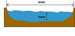
Figure \(\PageIndex{1}\) is a cross-sectional view of a lake basin illustrating two basic dimensions used to describe lakes: width and depth.

A horizontal arrow extends across the lake from one shoreline to the other and is labeled Width. This arrow represents the distance across the lake at the water surface.

A vertical arrow extends from the water surface down to the lake bottom and is labeled Depth. This arrow represents the vertical distance between the surface of the water and the deepest part of the basin.

The lake occupies a depression in the landscape, with sloping sides descending from the shoreline to the deeper central portion of the basin. The water fills the basin above the lake floor. The diagram introduces two fundamental measurements used to describe lake morphology:

• Width measures the horizontal extent of the lake.
• Depth measures the vertical distance from the water surface to the bottom.

These dimensions influence many lake characteristics, including water storage capacity, temperature patterns, mixing, aquatic habitat distribution, and biological productivity. Deeper lakes generally store more water and may develop layered temperature zones, while wider lakes often experience greater wind-driven circulation.

The cross-sectional area of the stream, shown in Figure \(\PageIndex{1}\), is determined by multiplying channel depth by channel width along a transverse section of the stream. For a hypothetical stream with a rectangular cross-sectional shape (a stream with a flat bottom and vertical sides) the cross-sectional area (A) is simply the width multiplied by the depth:

A = (W * D)

The wetted perimeter is the portion of the channel that is "wet". The wetted perimeter (WP) is the width plus twice the depth that the water touches:

WP= W + 2D

The greater the cross-sectional area in comparison to the wetted perimeter, the more freely flowing will the stream be because less of the water is in proximity to the frictional bed. So as hydraulic radius increases so will velocity (all other factors being equal).

Studies have shown that width and depth tend to vary regularly with stream discharge. If discharge is held constant and width decreases, then the channel should deepen by scouring. This occurs as a result of the increased velocity and transportation power which accompanies the narrowing of a channel. Studies have also shown that as mean discharge of a stream increases downstream so do channel width, depth, and average current velocity.

The flow velocity is directly related to the hydraulic radius (cross-sectional area divided by the wetted perimeter) and channel slope, and inversely related to channel roughness.

Channel slope or gradient is the difference in elevation between two points on a stream divided by the distance between them measured along the stream channel. The flow velocity, and thus power of the stream to do work is also directly related to the slope of the channel, the steeper the slope, the faster the velocity of flow.

Stream Flow

Sources of Stream Flow

There are four basic sources of stream flow which are illustrated in Figure \(\PageIndex{2}\). Groundwater flow into the channel is what provides for the base flow, or normal flow of the stream. For perennial streams the water table is at the height of the surface of the stream as shown below. The base flow of the stream is augmented by interflow from the soil moisture zone. At the surface, direct channel precipitation and surface runoff as overland flow contribute to stream flow during and following storms.

Figure \(\PageIndex{2}\): Sources of Stream Flow. (CC BY-SA 4.0 ; Curated by Michael Ritter via The Physical Environment).

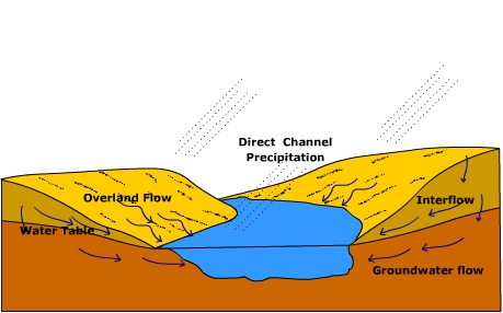
Figure \(\PageIndex{2}\) is a cross-sectional view of a watershed and stream system, showing the pathways by which water reaches a lake, pond, or stream channel after precipitation.

At the center of the figure is a blue surface-water body surrounded by sloping hillsides. Several arrows indicate the movement of water through and across the landscape.

Direct Channel Precipitation -Diagonal dashed lines represent rainfall falling directly onto the water body. This pathway is labeled Direct Channel Precipitation. Water falling directly into the stream, pond, or lake immediately contributes to streamflow without first moving across the land surface or through the soil.

Overland Flow - On the left hillside, arrows moving downslope across the ground surface are labeled Overland Flow. Overland flow occurs when rainfall exceeds the soil's infiltration capacity or when the soil is saturated. Water flows across the land surface directly into the channel, contributing to runoff and potentially increasing flood peaks.

Interflow - Within the upper soil layer on the right hillside, arrows move laterally through the soil toward the water body. This pathway is labeled Interflow. Interflow is the sideways movement of water through the shallow soil layers above the water table. It provides a delayed contribution to streamflow compared with overland flow.

Groundwater Flow - At the bottom of the figure, arrows move through the saturated zone toward the water body. This pathway is labeled Groundwater Flow. Groundwater flow represents water moving slowly through the saturated subsurface. It supplies baseflow to streams and helps maintain water levels during dry periods.

Water Table- A curved line beneath the surface is labeled Water Table. The water table marks the upper boundary of the saturated zone. Below this line, pore spaces are filled with groundwater; above it, soil contains both air and water.

The diagram illustrates the major pathways by which precipitation becomes streamflow:

• Direct precipitation adds water directly to the channel.
• Overland flow delivers rapid surface runoff.
• Interflow transfers water through shallow soil layers.
• Groundwater flow provides slower, sustained contributions from the saturated zone.

Flow velocity

Figure \(\PageIndex{3}\): Flow velocity. (CC BY-SA 4.0 ; Curated by Michael Ritter via The Physical Environment).

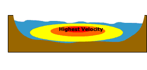
Figure \(\PageIndex{3}\) is a cross-sectional view of a stream channel showing how water velocity varies across the channel.The channel has sloping sides and a curved bottom. Water fills the channel, with the water surface at the top and the stream bed and banks forming the boundaries. A series of colored zones are shown within the water:

• A red region near the center of the channel is labeled “Highest Velocity.”
• Surrounding the red region is a yellow zone representing relatively high velocities.
• Areas closer to the stream bed, banks, and water surface are shown in blue, indicating lower velocities.

The region of highest velocity is located slightly below the water surface and near the center of the channel rather than directly at the surface or against the banks. 

The flow velocity of a stream, illustrated in Figure \(\PageIndex{3}\), is how fast the water is moving through a cross-section. Flow velocity is determined by the balance between the down slope gravitational stress as a result of the slope of the stream, and the loss or expenditure of energy in overcoming the frictional resistance of the channel bed and side. In general, the flow velocity is greatest at the center of the channel, just below the surface. More specifically the highest velocity of flow follows the stream thalweg, a line that connects the deepest part of the stream channel. Here, water moving through the stream encounters the least resistance to flow yielding a higher velocity of flow.

Flow Regimes

Under very low velocities water flows through a stream as smooth sheets running parallel to the bed called laminar flow. Laminar flow has an appearance much like that of a deck of cards with the top card jutting forward over those below. The tug of the channel bottom slows the water near the bed with the water nearer the surface flowing somewhat faster. Only the finest particles kind be detached, so laminar flow is basically nonerosive.

Under higher flow velocities, resistance within the flow and that caused by the bed and sides of the channel cause the flow to break down into separate currents. The swirling currents of turbulent flow undergo constant variation in speed and direction of flow. The swirls of water created during turbulent flow are more erosive than laminar flow and help suspend material in the stream. Turbulent flow is the "normal" type of flow in most streams.

Stream discharge

Stream discharge is the volume of water passing through a particular cross-section in a unit of time, measured in units like cubic meters per second or cubic feet per second. The discharge of a perennially flowing stream is provided by the influx of groundwater into the channel. This influx provides what is called the "base flow" of the stream. Water is added to the stream by runoff from the surrounding terrain during storm events.

Discharge(Q) can be expressed as

Q = A X V

where,

A= cross-sectional area

V= velocity

Figure \(\PageIndex{4}\): A stream hydrograph. (CC BY-SA 4.0 ; Curated by Michael Ritter via The Physical Environment).

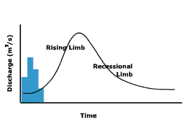
The hydrograph, shown in Figure \(\PageIndex{4}\), is a graphical way of portraying the change in discharge over time, and how it relates to inputs of water and the environment in which the stream is located. The Y-axis of the hydrograph is scaled for discharge, and when investigating the influence of a storm event, precipitation. The X-axis is scaled for time. Discharge is plotted as a line and precipitation as a bar graph. The hydrograph shows discharge starting at its base flow, rising to a peak (the rising limb) and then declining (recessional limb) back to its base flow. Notice how the peak in precipitation does not occur at the same time as the peak in discharge. In other words, there is a lag period between the time when the most precipitation occurs and when the most discharge is recorded.

A number of factors influence the shape of the hydrograph and the length of the lag period. Elongate basins tend to exhibit flatter hydrographs because it takes a longer time for water to move from the head to the recording station at the mouth of the basin. Travel time is less for circular basins resulting in a more peaked hydrograph.

Figure \(\PageIndex{5}\): Comparison of pre-urban and post-urban watershed discharge. (CC BY-SA 4.0 ; Curated by Michael Ritter via The Physical Environment).

Figure \(\PageIndex{5}\) is a graph that compares streamflow after a rainfall event in urban and preurban environments. Blue bars represent precipitation over time. The urban hydrograph rises rapidly, reaches a higher peak discharge, and has a shorter lag time between rainfall and peak flow. The preurban hydrograph rises more gradually, reaches a lower peak discharge, and has a longer lag time. The diagram demonstrates that urbanization increases surface runoff and speeds the movement of water into streams, resulting in faster and larger flood peaks compared with preurban conditions.

Land cover is another important control over the shape of a stream hydrograph. Figure \(\PageIndex{5}\) provides a comparison of pre-urban and post urban watershed discharge. Under natural conditions, vegetation slows surface runoff and encourages infiltration. As a result, the hydrograph is less peaked and the lag time is longer than a basin with little vegetation. Urbanization of a watershed can have a drastic effect on runoff, discharge, and the resulting hydrograph. Urbanization replaces permeable surface with impermeable ones, streets, parking lots, buildings etc. Water runs off the surface more efficiently and is diverted to nearby streams by the construction of storm sewers. Storm sewers effectively increase the urbanized watershed drainage density. As a result, urbanized watersheds tend to exhibit more peaked hydrographs with shorter lag periods.

Stream energy

The energy that a stream possesses is closely related to its discharge because discharge determines flow velocity. Flow velocity controls the stream's capacity to erode and transport sediment through its channel. Generally, the larger the discharge, the smoother the channel, greater the stream velocity. Cross-sectional area and discharge increases down stream due to tributary and ground water flow into the channel. As a result, one might expect flow velocity to increase in the down stream direction as well. However, as streams grow larger their down stream slope decreases, preventing a continuous buildup of energy and creating a more uniform distribution of stream energy along its length.

Floods and Flooding

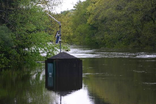
A flood occurs when a stream channel can no longer contain the water moving through it. Floods usually are local, short-lived events, others can be catastrophic, happening with little or no warning. Floods are most often caused by prolonged rainfall that saturates the ground causing surface runoff into nearby streams increasing their discharge. Flooding occurs when the water spills out of the channel and on to the adjacent terrain. Though viewed as a "natural hazard" to humans, flooding is a natural, rejuvenating process. Figure \(\PageIndex{6}\) shows a stream flow gauge on the Lamprey river near New Market, New Hampshire.

Figure \(\PageIndex{6}\): Stream Flow Gauge on the Lamprey River near Newmarket, NH. (CC BY-SA 4.0 ; Curated by Michael Ritter via The Physical Environment).

Causes and Conditions

Generally speaking there are two types of floods:

1. where water slowly rises and spills over the banks of a stream or river
2. flash floods.

Floods can occur at anytime of year, but particular seasonal weather patterns are more conducive to the creation of floods than others in different geographic regions. In the United States, cyclonic storms roaring off the ocean and into the Pacific coast states during the winter and early spring can cause flooding. Figure \(\PageIndex{7}\) maps the flood season for United States. In the southwest, summer and fall thunderstorms release torrents of water that rush down dry stream beds or arroyos as flash floods. Flooding can occur in the north central states during the winter as rain fall or snow melt runs off the frozen ground surface, or ice jams rivers causing them to flood. Flooding in the mid portion of the United States tends to occur in spring and summer as polar front cyclones march across the North American continent. Hurricanes and large convective complexes create flooding in the late summer and fall along the Gulf coast of the United States.

Figure \(\PageIndex{7}\): Flood Season in the United States. (CC BY-SA 4.0 ; Curated by Michael Ritter via The Physical Environment).

Figure \(\PageIndex{7}\) is the map of the United States shows the timing of peak streamflow, or the season when rivers and streams typically experience their highest discharge. Curved boundary lines divide the country into regions labeled by season.

Winter Peak Flow - In these areas, streamflow peaks during winter because most precipitation falls as rain and quickly enters rivers. Regions labeled Winter occur primarily along:

• The Pacific Northwest coast
• Parts of California
• Portions of the western mountains

Early Spring Peak Flow - These regions experience peak flows shortly after winter due to a combination of rainfall and early snowmelt. Regions labeled Early Spring are found in:

• Parts of the Pacific Northwest interior
• Portions of the central and southern Rocky Mountains
• Parts of the central United States

Spring Peak Flow - Peak streamflow occurs in spring as rainfall increases and accumulated winter snow melts. Areas labeled Spring include:

• Much of the Great Plains
• Parts of the Mississippi River basin
• Portions of the eastern United States

Late Spring - A narrow band across portions of the northern United States and high-elevation western regions is associated with Late Spring peak flow. Snowmelt continues later into the year because of colder temperatures and higher elevations.

Summer Peak Flow - Peak flow is often associated with delayed mountain snowmelt or intense summer rainfall. Regions labeled Summer occur in:

• Parts of the northern Rocky Mountains
• Sections of the central United States
• Portions of the Gulf Coast region

Late Summer and Fall Peak Flow - Peak flows in these regions are often linked to seasonal thunderstorms and monsoon rainfall. Areas labeled Late Summer and Fall are found primarily in:

• The desert Southwest
• Arizona and New Mexico
• Portions of the western United States

Fall Peak Flow - Peak discharge occurs during autumn due to seasonal rainfall patterns and tropical storm activity. The Fall region is concentrated in:

• Florida
• Portions of the southeastern United States

In tropical regions like Bangladesh, monsoon rains saturate the ground causing severe flooding. Europe floods from the sea may occur as a result of Atlantic storms pushing water to the coast and can be particularly damaging when occurring at high tide. Deforestation greatly increases the risk for flooding.

Figure \(\PageIndex{8}\): A family standing on a raised platform during floods. (CC BY-SA 4.0; Courtesy Hansel Ohioma via Wikimedia Commons).

Some of the worst flooding in decades also occurred during the summer of 2007. Flooding in Britain was caused by a persistent jet stream sitting further south than usual at this time of the year. System after system pounded the British Isles. During August of 2007, widespread flooding occurred in the Midwest United States causing damage exceeding $115 million. Figure \(\PageIndex{9}\) illustrates the axis of rain during the historic rainfall and flooding event in Minnesota on 18th August 2007. A warm front advanced northward into Iowa and Illinois during mid-August where it stalled and became a stationary front. Warm, moist air overrunning the front provided the ingredients for showers and thunderstorms. Rainfall over the weekend of August 18-19, 17 inches of precipitation fell in Witoka, MN. Rochester, MN measured 6.9 inches of rainfall. The heavy rain sent streams in the region over their banks. Moisture from Tropical Storm Erin to the south enhanced the stormy conditions.

Figure \(\PageIndex{9}\): Weather Conditions in Minnesota during the historic rainfall and flooding event in of August 18-20, 2007. (CC BY-SA 4.0 ; Curated by Michael Ritter via The Physical Environment).

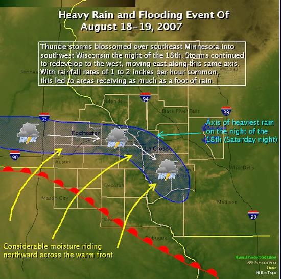
Figure \(\PageIndex{9}\) is a weather map showing the heavy rain and flooding event of August 18–19, 2007, affecting southeastern Minnesota and southwestern Wisconsin.

At the top of the map is a title: “Heavy Rain and Flooding Event of August 18–19, 2007.” A text box explains that thunderstorms repeatedly developed and moved along the same path during the night of August 18, producing rainfall rates of 1 to 2 inches per hour, with some locations receiving up to a foot of rain.

The map covers parts of Minnesota, Wisconsin, and Iowa, with cities such as Rochester, La Crosse, Black River Falls, Austin, and Decorah labeled. Interstate highways including I‑90, I‑94, and I‑39 are also shown.

Several weather features are illustrated:

• A warm front extends across southern Iowa and northern Illinois, shown by a curved red line with semicircles.
• Large yellow arrows point northward from the south, labeled “Considerable moisture riding northward across the warm front.” These arrows represent warm, moisture-rich air moving into the region.
• Thunderstorm symbols mark areas of intense rainfall.
• White arrows indicate the movement of storm cells.
• A blue shaded corridor stretches across southeastern Minnesota into western Wisconsin, highlighting the storm track.

A bright blue label identifies the “Axis of heaviest rain on the night of the 18th (Saturday night)” near the La Crosse area. This axis marks the zone where repeated storms moved over the same locations, producing extreme rainfall totals.

The map explains the meteorological conditions that led to severe flooding. Moist air moving northward across a warm front fueled persistent thunderstorms. Because storms repeatedly formed and traveled along the same path, large amounts of rain fell over a relatively narrow corridor. This process concentrated rainfall in specific areas, causing flooding and unusually high runoff. The figure demonstrates how storm track, moisture transport, and frontal systems can combine to produce extreme precipitation events.

Flood Frequency

Figure \(\PageIndex{10}\): 100-Year Flood Plain. (CC BY-SA 4.0 ; Curated by Michael Ritter via The Physical Environment).

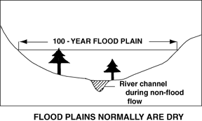
Figure \(\PageIndex{10}\) is a cross-sectional view of a river valley and its floodplain.

At the center of the valley is a narrow river channel during non-flood flow, shown as a small channel incised into the valley floor. Under normal conditions, water remains confined within this channel.

A broad, relatively flat area extends on both sides of the river channel. An arrow spanning this flat surface is labeled “100-Year Flood Plain.” This area represents the portion of the valley that has a 1% chance of being flooded in any given year.

Two trees are shown growing on the flat valley floor, illustrating that the floodplain is normally dry land and may support vegetation, agriculture, or human development. A note at the bottom states “Flood plains normally are dry.”

The valley sides rise upward from the floodplain, forming higher ground that is less likely to be inundated during floods.

The diagram illustrates the relationship between a river channel and its floodplain. During normal flow, water remains within the river channel. During major flood events, however, water can spread across the surrounding floodplain, temporarily covering areas that are usually dry.

The 100-year floodplain identifies land that is susceptible to infrequent but significant flooding and is commonly used in flood-risk assessment, land-use planning, and development decisions. The figure emphasizes that although floodplains appear stable and dry most of the time, they are part of the river system and can periodically become inundated during large floods.

Using frequency analysis, one can estimate the probability of the occurrence of a given flood event The recurrence interval, also known as the return period, is based on the probability that the given event will be equaled or exceeded in any given year. For instance, a one hundred year flood has a 1% chance of occurring in any given year. One hundred year floods are rare but can be devastating. The 100-year flood plain as shown in Figure \(\PageIndex{10}\), is used for flood plain management and insurance purposes. Those living within this zone are often required to have flood insurance in addition to their regular home owner's insurance.

Figure \(\PageIndex{11}\): Development of flood plains increases risk of floods. (CC BY-SA 4.0 ; Curated by Michael Ritter via The Physical Environment) 

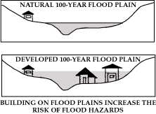
Figure \(\PageIndex{11}\) contains two cross-sectional diagrams comparing a natural floodplain with a developed floodplain.