10.1: The Stream System

Drainage Basins and Stream Systems

The fundamental unit of study for fluvial processes is the drainage basin or watershed. A drainage basin is a portion of the Earth's surface that contains a main stream and its tributaries and is bounded by a drainage divide. As illustrated in Figure \(\PageIndex{1}\), the drainage divide represents the boundary between adjacent drainage basins and determines into which basin precipitation flows. There is no upper or lower limit to the size of a drainage basin. We can delimit the drainage basin of the Mississippi River as most of the area east of the Rocky Mountains. Figure \(\PageIndex{2}\) highlights the drainage basin of the Mississippi River and its tributaries are rivers like the Missouri, Arkansas, and Ohio to name just a few.

Figure \(\PageIndex{1}\): The Drainage Basin. (CC BY-SA 4.0; Courtesy Michael Ritter in The Physical Environment).

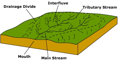
 Figure \(\PageIndex{1}\) is a three-dimensional block model of a drainage basin (watershed) showing the major components of a stream system.

At the center of the landscape is a larger channel labeled Main Stream. The main stream flows through the basin and exits at a location labeled Mouth, where water leaves the drainage basin.

Several smaller channels branch across the landscape and flow into the main stream. One of these is labeled Tributary Stream. Tributaries collect runoff from smaller areas and deliver water to the main stream.

The higher land between neighboring tributary valleys is labeled Interfluve. Interfluves form ridges or upland areas that separate adjacent tributary channels.

The outer boundary of the watershed is marked by a ridge labeled Drainage Divide. The drainage divide separates this drainage basin from neighboring basins. Precipitation falling on one side of the divide flows into this basin, while precipitation falling on the opposite side flows into a different drainage basin.

The stream channels branch in a pattern resembling tree limbs, converging toward the main stream and eventually toward the mouth.

The diagram illustrates the structure of a drainage basin, the fundamental unit used to study fluvial systems. It shows how precipitation and runoff are collected by tributaries, transferred to a main stream, and carried out of the basin through the mouth. The drainage divide defines the watershed boundary, while interfluves separate neighboring tributary systems. Together, these features demonstrate how water is organized and transported within a river network.

Figure \(\PageIndex{2}\): Mississippi River Basin. (Public Domain ; Courtesy National Parks Gallery Source Picryl).

Figure \(\PageIndex{2}\) shows the Mississippi River drainage basin (watershed), one of the largest drainage basins in North America.

A dashed line outlines the watershed boundary, enclosing a vast region that covers much of the central and eastern United States. The boundary marks the drainage divide separating the Mississippi Basin from neighboring watersheds. Any precipitation falling inside this boundary ultimately flows toward the Mississippi River system.

The Mississippi River runs from the upper central United States southward to the Gulf of Mexico and serves as the main stream of the basin. Several major tributaries are labeled:

• Missouri River, entering from the west and draining much of the Great Plains and Rocky Mountain region.
• Arkansas River, flowing eastward from the Rocky Mountains into the lower Mississippi.
• Ohio River, joining the Mississippi from the east and draining a large portion of the eastern United States.

Numerous smaller tributaries, shown as branching blue lines, feed into these major rivers, creating a tree-like drainage network.

The map highlights how water collected across a large portion of the continent is funneled through interconnected tributaries into the Mississippi River and ultimately discharged into the Gulf of Mexico.

Streams within the drainage basin are either perennial or intermittent in flow. Perennial streams flow all year. Glacier fed streams are examples of perennial streams. The river Ganges in India is an example of a perennial river and is made up of meltwater from the Gangotri Glacier.Figure \(\PageIndex{3}\) shows a photograph of River Ganges that was taken near the town of Hrishikesh in India.  River Nile in Africa is a perennial river with its tributaries providing it water and maintaining stream flow all year round. The primary water source for the river Mississippi, a perennial river in U.S.A is Lake Itasca in northern Minnesota.  The base flow of these streams is provided by groundwater seepage into the channel. Tributary streams are small streams that enter into the main stream. Tributary streams, especially the smaller ones around the periphery of the basin, are intermittent. Intermittent streams only flow during wetter times of the year. Much of their flow is provided by surface runoff and when the water table is higher as a result of moist conditions. The upland between tributaries is called an interfluve. Generally they have low stream flow during dry season. Rivers in western Namibia like Ugab and Swakop are examples of intermittent or non perennial rivers. 

Figure \(\PageIndex{3}\): River Ganges near Hrishikesh. (CC BY-SA 4.0; Courtesy Aditya Katiyar via Wikimedia Commons).

Some streams are classified as exotic streams. Exotic streams are those that originate in a humid region but flow through an arid region. Such is the case of the Nile and Colorado Rivers. The headwaters of the Nile River is in the wet Ethiopian Highlands, and travels through the eastern portion of the Sahara Desert on its way to the Mediterranean Sea. Along its route, the river loses substantial amounts of water to evaporation. The same is true for the Colorado River shown in Figure \(\PageIndex{4}\). With its headwaters in the Rocky Mountains, it flows south and west towards the southwest desert of the United States. During its journey it loses nearly half its flow to evaporation. The Colorado used to flow to the ocean, astonishingly it no longer does. The river is originally a perennial river, however due to excessive damming the lower courses often turn completely dry before reaching the Gulf of Colombia. Dams built have been used to divert water for agriculture and municipal use. 

Figure \(\PageIndex{4}\): Course of the Colorado River, U.S.A. (CC BY-SA 4.0; Shannon1 via Wikimedia Commons).

 Figure \(\PageIndex{4}\) shows the Colorado River drainage basin in the southwestern United States and northwestern Mexico. The Colorado River is highlighted as the main river system, with numerous tributaries branching into it from surrounding states.

The basin extends across parts of Wyoming, Colorado, Utah, New Mexico, Arizona, Nevada, California, and Mexico. The main channel of the Colorado River begins in the Rocky Mountains of Colorado and flows southwest through the Grand Canyon before reaching the Colorado River Delta near the Gulf of California.

Major tributaries labeled on the map include:

• Green River, the largest tributary, flowing south from Wyoming through Utah.
• Yampa River
• White River
• Gunnison River
• San Juan River
• Dolores River
• Little Colorado River
• Virgin River
• Gila River

Numerous reservoirs are also shown, including:

• Lake Powell
• Lake Mead
• Lake Mohave
• Lake Havasu
• Flaming Gorge Reservoir
• Navajo Lake

Several major cities are marked for reference, including Denver, Salt Lake City, Las Vegas, Phoenix, Grand Junction, Flagstaff, and Yuma.

The drainage network has a branching, tree-like pattern in which smaller tributaries flow into larger streams, eventually joining the Colorado River. The boundaries of the watershed are defined by surrounding mountain ranges and highlands that separate this basin from neighboring drainage basins, such as the Rio Grande Basin to the east.

Drainage Patterns

Figure \(\PageIndex{5}\): Satellite Image of the Eastern Desert with a view of Rive Nile exhibiting dendritic drainage pattern. (CC BY-SA 3.0 IGO; Contains modified Copernicus Sentinel data via Wikimedia Commons).

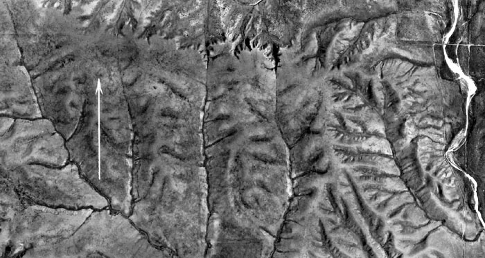
Over time, a stream system achieves a particular drainage pattern to its network of stream channels and tributaries as determined by local geologic factors. Drainage patterns or nets are classified on the basis of their form and texture. Their shape or pattern develops in response to the local topography and subsurface geology. Drainage channels develop where surface runoff is enhanced and earth materials provide the least resistance to erosion. The texture is governed by soil infiltration, and the volume of water available in a given period of time to enter the surface. If the soil has only a moderate infiltration capacity and a small amount of precipitation strikes the surface over a given period of time, the water will likely soak in rather than evaporate away. If a large amount of water strikes the surface, then more water will evaporate, soak into the surface, or ponds on level ground. On sloping surfaces this excess water will runoff. Fewer drainage channels will develop where the surface is flat and the soil infiltration is high because the water will soak into the surface. The fewer number of channels, the coarser will be the drainage pattern.

Figure \(\PageIndex{5}\) shows satellite image of the Eastern Desert in central-eastern Egypt, between the Nile River and the Red Sea. The image shows a barren, arid landscape with visible water erosion patterns. Here dendritic drainage pattern is clearly visible. The Nile River valley is at the bottom of the image, appearing red due to false-color processing, with black dots representing cities and towns.

Figure \(\PageIndex{6}\): Dendritic drainage pattern. (CC BY-SA 4.0 ; Courtesy Michael Ritter via The Physical Environment).

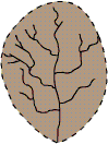
A dendritic drainage pattern, shown in Figure \(\PageIndex{6}\) is the most common form and looks like the branching pattern of tree roots. It develops in regions underlain by homogeneous material. That is, the subsurface geology has a similar resistance to weathering so there is no apparent control over the direction the tributaries take. Tributaries joining larger streams at acute angle (less than 90 degrees). 

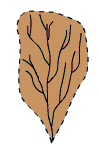
Parallel drainage patterns, illustrated in Figure \(\PageIndex{7}\) form where there is a pronounced slope to the surface. A parallel pattern also develops in regions of parallel, elongate landforms like outcropping resistant rock bands. Tributary streams tend to stretch out in a parallel-like fashion following the slope of the surface. A parallel pattern sometimes indicates the presence of a major fault that cuts across an area of steeply folded bedrock. All forms of transitions can occur between parallel, dendritic, and trellis patterns. 

Figure \(\PageIndex{7}\): Parallel drainage pattern. (CC BY-SA 4.0 ; Courtesy Michael Ritter via The Physical Environment).

Trellis drainage patterns shown in Figure \(\PageIndex{8}\) look similar to their namesake, the common garden trellis. Trellis drainage develops in folded topography like that found in the Appalachian Mountains of North America. Down-turned folds called synclines form valleys in which resides the main channel of the stream. Short tributary streams enter the main channel at sharp angles as they run down sides of parallel ridges called anticlines. Tributaries join the main stream at nearly right angles. 

Figure \(\PageIndex{8}\): Trellis Drainage Pattern. (CC BY-SA 4.0 ; Courtesy Michael Ritter via The Physical Environment).

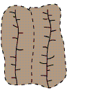
The rectangular drainage pattern illustrated in Figure \(\PageIndex{9}\) is found in regions that have undergone faulting. Streams follow the path of least resistance and thus are concentrated in places were exposed rock is the weakest. Movement of the surface due to faulting off-sets the direction of the stream. As a result, the tributary streams make sharp bends and enter the main stream at high angles.

Figure \(\PageIndex{9}\): Rectangular Drainage Pattern. (CC BY-SA 4.0 ; Courtesy Michael Ritter via The Physical Environment).

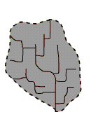
Figure \(\PageIndex{10}\) illustrates the radial drainage pattern develops around a central elevated point. This pattern is common to such conically shaped features as volcanoes. The tributary streams extend the headward reaches upslope toward the top of the volcano

Figure \(\PageIndex{10}\): Radial Drainage Pattern. (CC BY-SA 4.0 ; Courtesy Michael Ritter via The Physical Environment).

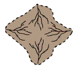
The centripetal drainage pattern shown in Figure \(\PageIndex{11}\) is just the opposite of the radial as streams flow toward a central depression. This pattern is typical in the western and southwestern portions of the United States where basins exhibit interior drainage. During wetter portions of the year, these streams feed ephemeral lakes, which evaporate away during dry periods. Salt flats are created in these dry lake beds as salt dissolved in the lake water precipitates out of solution and is left behind when the water evaporates away.

Figure \(\PageIndex{11}\): Centripetal Drainage Pattern. (CC BY-SA 4.0 ; Courtesy Michael Ritter via The Physical Environment).

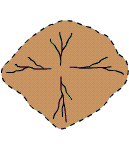
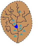
Deranged or contorted patterns develop from the disruption of a pre-existing drainage pattern. Figure \(\PageIndex{12}\) began as a dendritic pattern but was altered when overrun by glacier. After receding, the glacier left behind fine grain material that form wetlands and deposits that dammed the stream to impound a small lake. The tributary streams appear significantly more contorted than they were prior to glaciation.

Figure \(\PageIndex{12}\): Deranged Drainage Pattern. (CC BY-SA 4.0 ; Courtesy Michael Ritter via The Physical Environment).

The patterns described above are accordant, or correlated with the structure and relief over which they flow. Those streams that are discordant with the rocks over which they flow are either antecedent or superimposed. For instance, antecedent streams flowed across bedrock structures prior to uplift. Slow mountain building permitted stream erosion to keep pace with uplift. Such appears to be the case for the Columbia River that cuts across the Cascade Mountains. Streams in portions of the Appalachian Mountains have formed in weaker rock that through time has eroded away. These streams appear to be superimposed over the rock layers that they presently flow over. The Cumberland Gap is a famous water gap formed in this way as it cuts through the folds of the Appalachians.