5.11: Urban Climate

Cities and Climate

Urbanization has a significant impact on all elements of the atmosphere. Replacing natural vegetation with artificial surfaces alters the heat balance and hydrology of the local environment. Urban canyons affect wind speed and increased particulate content enhances precipitation down wind of a city.

Figure \(\PageIndex{1}\): Urban Heat Island. (CC BY-SA 4.0; Michael Ritter via The Physical Environment).

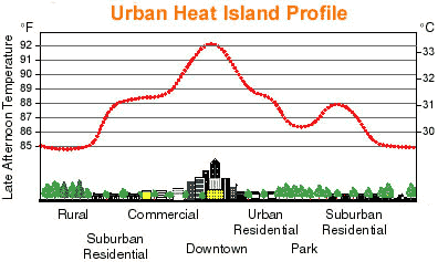
Figure \(\PageIndex{1}\) is titled “Urban Heat Island Profile.”

The graph illustrates how air temperature varies across different land-use zones from a rural area, through a city center, and back to suburban areas.

The horizontal axis shows a sequence of environments:

• Rural
• Suburban Residential
• Commercial
• Downtown
• Urban Residential
• Park
• Suburban Residential

The vertical axes show temperature in both degrees Fahrenheit (left) and degrees Celsius (right).

A line represents air temperature across the landscape.

• Temperatures begin at their lowest levels in the rural area, around 85°F (30°C).
• Temperatures increase through the suburban residential and commercial zones.
• The highest temperature occurs in the downtown area, reaching approximately 92°F (33°C).
• Temperatures decline through the urban residential area.
• A noticeable cooling occurs over the park, where temperatures drop several degrees below surrounding urban areas.
• Temperatures rise slightly in the second suburban residential area before decreasing again toward rural values.

Illustrations along the bottom show land-cover differences, including trees in rural and suburban areas, dense buildings in the downtown core, and green space within the park.

The concentration of human activities in urban areas creates an "island" of heat surrounded by a "sea" of cooler rural areas called the urban heat island. Heat is added to the urban atmosphere by industry, transportation, exhaust heat, and air conditioning among other things. Artificial surfaces with low albedo absorb much insolation, heating the surface more than if it were a natural surface like grass. The additional heat can create differences in air temperature between the city and countryside of 10^oC (18^oF) or more. Consequently, snow disappears earlier and vegetation bloom earlier in the city. Sunlight is trapped within the "urban canyon" by reflective surfaces. Building materials like brick and asphalt have high heat conductivity. Heat loss in the evening can compensate for that which has been gained during the day.

Figure \(\PageIndex{2}\): Typical albedos. (CC BY 4.0; Image created by OpenAI ChatGPT. (2026))

In Figure \(\PageIndex{2}\) we observe that a cross-sectional landscape compares a densely built city center with surrounding rural fields and parks. A red-orange heat dome covers the city, illustrating that urban air temperatures can be up to 10°C (18°F) warmer than the nearby countryside. Arrows show heat entering the urban atmosphere from industry, transportation, vehicle exhaust, and air conditioning. Additional arrows show sunlight being absorbed by dark, low-albedo surfaces such as asphalt, brick, concrete, and dark roofs, while reflective building walls trap sunlight within an urban canyon. A comparison chart lists approximate albedo values: dark asphalt 0.05–0.10, black roof 0.05–0.13, gravel roof 0.10–0.15, brick 0.15–0.25, concrete 0.20–0.35, glass 0.10–0.25, grass 0.25–0.30, trees 0.15–0.25, white roof 0.60–0.80, light concrete 0.40–0.60, and water 0.05–0.10. Lower panels compare daytime heat gain and nighttime heat release, showing that cities retain heat longer than rural areas. Final panels illustrate earlier snowmelt and earlier spring vegetation blooming in urban environments because of warmer temperatures.

The warm city surface induces convection that draws urban air upwards, which is then replaced by cool air from the countryside. This rural-urban circulation is more likely to occur when synoptic-scale winds are light. The rising air transports dust and other particulates upward, gathering as a dust dome. If synoptic-scale winds are strong enough, the pollutants spill over the city boundary and stretch downwind over the countryside as a pollution plume. Particulates concentrated in the urban atmosphere serve as nuclei for the condensation of water. Several studies have shown how precipitation is enhanced downwind of an urban area due to increased particulate content from urban sources.

In rural areas, more available water for evaporation keeps surface temperatures cooler. Impermeable artificial surfaces in the city increase water runoff and reduce infiltration. This results in less moisture available for evaporative cooling and higher sensible transfer than in the surrounding rural areas.

Figure \(\PageIndex{3}\): Atlanta, GA. urban heat island. False-color image, vegetation is red, urban areas blue to black. (CC BY-SA 4.0; Michael Ritter via The Physical Environment).

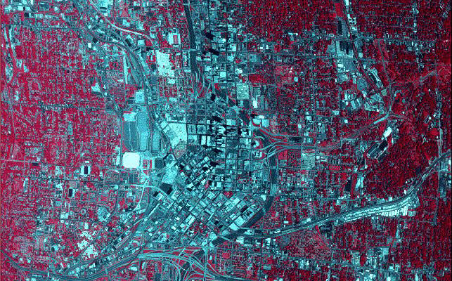
Figure \(\PageIndex{3}\) is a false-color satellite image of the Atlanta, Georgia metropolitan region. Healthy vegetation and forested areas appear in vibrant shades of red, dominating the surrounding landscape. In stark contrast, the heavily developed urban core, highways, and commercial zones show up as a sprawling network of blue, gray, and black signatures slicing through the center of the image. 

This false-color distribution has direct implications for the development and intensity of the Urban Heat Island (UHI) effect:

• Thermal Mass and Heat Storage: The extensive blue and black areas represent asphalt, concrete, and roofing materials. These dark, impervious surfaces have a low albedo, meaning they absorb and store massive amounts of shortwave solar radiation during the day and slowly re-radiate it as thermal infrared energy at night, keeping the urban core artificially warm.
• Loss of Evaporative Cooling: The vibrant red areas highlight where natural vegetation has been replaced by urbanization. Forests and fields naturally cool the air through evapotranspiration—a process where plants release moisture, absorbing latent heat. Removing this green cover eliminates a city's primary natural air conditioning mechanism.
• Microclimate Fragmentation: The sharp visual boundaries between the red (vegetated) and blue/black (built) zones show how urban sprawl creates distinct microclimates. The contiguous dark zones act as giant heat retention nodes, causing urban temperatures to spike significantly higher than the cooler, well-vegetated rural surroundings.