5.9.3: Midlatitude Steppe

Geographic Distribution 

Figure \(\PageIndex{1}\): Sheep grazing on grass the eastern confines of the Horquin Desert (Inner Mongolia). (CC BY-SA 4.0; Michael Ritter via The Physical Environment).

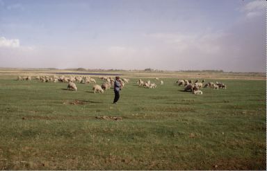
The midlatitude steppe climate shares many of the same characteristics that the tropical steppe has. Both are semi-arid climates that are affected by their interior continental or leeward orographic position. However, the midlatitude steppe experiences larger temperature ranges and receives more total rainfall than the tropical steppe climate.

Midlatitude steppes are found on the periphery of midlatitude deserts and the leeward side of mountain systems in inner Asia, South America, and the Western United States. Much of the Great Plains of the United States lies in the midlatitude steppe climate. Broad expanses of steppe climate run through Mongolia and Kazakhstan.

Controlling Factors

The controlling factors over the geographical distribution and climatic characteristics of the midlatitude steppe are similar to that of the midlatitude deserts. The climate is found in the interior of the vast midlatitudes continents of the Northern Hemisphere, far removed from sources of moisture. Midlatitude steppe climate is located in the rain shadow of tall mountain chains like the Rocky and Andes Mountains in North and South America respectfully. These mountain systems act as a barrier to westerly flowing moist air.

Figure \(\PageIndex{2}\): Climograph for Hohot, China (CC BY-SA 4.0; Michael Ritter via The Physical Environment).

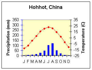
Figure \(\PageIndex{2}\) is a climate graph for Hohhot, China. The horizontal axis shows the months January through December. The left vertical axis is labeled “Precipitation (mm)” and ranges from 0 to 350 millimeters. The right vertical axis is labeled “Temperature (°C)” and ranges from approximately −25°C to 35°C.

In Figure \(\PageIndex{2}\), the horizontal axis shows the months January through December. The left vertical axis is labeled “Precipitation (mm)” and ranges from 0 to 350 millimeters. The right vertical axis is labeled “Temperature (°C)” and ranges from approximately −25°C to 35°C.

Precipitation is represented by blue bars. Rainfall is low during winter and spring, increases sharply in early summer, and peaks during July and August, when monthly precipitation exceeds 100 millimeters. Rainfall then declines through autumn.

Temperature is represented by a red line with diamond markers. Temperatures are very cold in winter, below −10°C in January, rise steadily through spring to a summer peak near 25°C in July, and then decrease rapidly through autumn and winter. 

Basic conclusions from the Climograph are as follows:

Average Annual Temperature (C) = 6.1
Annual Temperature Range (C) = 35.5
Total Annual Precipitation (mm) = 404.6
Summer Precipitation (mm) =362.8
Winter Precipitation (mm) = 44.1

Distinguishing Characteristics

Temperature

Temperature in the midlatitude steppe climate varies considerably with latitude, elevation, and continentality. Temperatures can range from -40^oC (-40^oF) in winter to above 40^oC (104^oF) in summer. Due to their continental position, the steppe climates of the northern Great Plains and Siberia generally experience the lowest temperatures of this climate. As one might expect, temperature increases as one travels toward the equatorward margin of the climate. Cooler temperatures also prevail as one moves toward high elevation. The temperature range for central Asian locations can be as much as 40^oC (22^oF), yet along the Argentine coast as small as 12^oC (6.7^oF). This extreme continentality is vividly illustrated in locations like Hohhot, China, where the annual temperature range swings across a dramatic 35.5°C between deeply frozen winters and warm summers (shown in Figure \(\PageIndex{2}\)).Though places like Santa Cruz, Argentina (shown in Figure \(\PageIndex{3}\)) have a moderately small temperature range due to their near-coastal location, they lie in the rain shadow of the Andes and hence experience very little precipitation.

Figure \(\PageIndex{3}\): Climograph for Santa Cruz, Argentina (CC BY-SA 4.0; Michael Ritter via The Physical Environment).

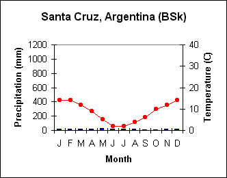
Figure \(\PageIndex{3}\) is a climate graph for Santa Cruz, Argentina, labeled “BSk”, indicating a cold semi-arid (steppe) climate.The horizontal axis shows the months January through December. The left vertical axis is labeled “Precipitation (mm)” and ranges from 0 to 1,200 millimeters. The right vertical axis is labeled “Temperature (°C)” and ranges from 0°C to 40°C. 

Precipitation is represented by blue bars. Rainfall is very low throughout the year, with only small monthly amounts and little seasonal variation.

Temperature is represented by a red line with circular markers. Temperatures are warmest during the Southern Hemisphere summer, near 14°C in January and December. Temperatures decline steadily through autumn, reaching a minimum of about 2°C to 4°C in June and July, before rising again through spring.

The basic elements from the climograph are : 

Average Annual Temperature (C) = 8
Annual Temperature Range (C) = 12
Total Annual Precipitation (mm) = 202
Summer Precipitation (mm) =94
Winter Precipitation (mm) = 104

Precipitation

With annual precipitation greater than half the annual potential evapotranspiration, the midlatitude steppe is considered a semi-arid climate. Precipitation ranges from 100 to over 300 mm in a year. There are few generalities that can be made about the precipitation regime of this climate. The seasonality of precipitation is similar to the nearest humid climate. Generally speaking, if the steppe climate borders the humid continental climate it is likely to have a summer maximum while bordering the humid subtropics a winter maximum may occur. Those steppe climates located closer to the coast may not have significant variability in their precipitation.