3.2.2: Explaining Patterns of Air Temperature

Factors affecting Global Air Temperature

Global patterns of air temperature are a reflection of the relative importance of sun angle and insolation intensity, day length, and location with respect to water bodies. We have found that low latitude locations experience less variation in sun angle and day length than do mid- and high latitude locations. Places located near large bodies of water tend to have more moderate temperatures than those further inland.Due to uneven heating of the earth air temperature varies spatially across the earth. Several key factors interact among themselves to influence the temperature of a particular location. The different factors are listed in this section summarizing some of the content learnt so far in this chapter. 

Latitude 

Because of the Earth's spherical shape, sunlight strikes the surface at different angles. The region around the Equator receives intense, concentrated heat because the sun shines directly or nearly directly on it throughout the year. Specifically, during the solstices, the sun’s direct rays hit their limit at the Tropic of Cancer in the north and the Tropic of Capricorn in the south. In areas outside these Tropics, the sun's rays arrive at a slant; this spreads solar energy over a larger surface area, significantly lowering the heat intensity. Based on this concept, the Greek philosopher Parmenides developed a system of climatic bands, which Aristotle later adopted and popularized in his work Meteorologica. They divided the Earth into five distinct bands classified into three temperature zones illustrated in Figure \(\PageIndex{1}\). 

The Torrid Zone

This is the central and hottest region. It extends north to the Tropic of Cancer and south to the Tropic of Capricorn. The concentration of direct sunlight here results in high temperatures and a tropical climate.

The Temperate Zones

There are two bands in this category. The North Temperate Zone lies between the Tropic of Cancer and the Arctic Circle, while the South Temperate Zone lies between the Tropic of Capricorn and the Antarctic Circle. Because sunlight reaches these areas at a slant, they experience moderate temperatures—neither extremely hot nor extremely cold.

The Frigid Zones

These regions are characterized by extremely low temperatures year-round because they receive the most slanted, low-intensity rays. The North Frigid Zone extends from the Arctic Circle to the North Pole, and the South Frigid Zone extends from the Antarctic Circle to the South Pole.

Figure \(\PageIndex{1}\): Temperature zones on the earth (CC BY-SA 4.0; Rajneesh kumar Thakur via Wikimedia Commons)

Figure \(\PageIndex{1}\) is titled “Temperature Zones of Earth.” It shows how the angle of incoming sunlight varies with latitude and creates different global temperature zones.

The Sun appears on the left, sending sunlight toward Earth on the right. A broad beam labeled “Direct sunlight” strikes the central part of Earth near the Equator. Another label, “Low angle of incoming sunlight,” points to sunlight reaching higher latitudes closer to the poles.

Earth is divided into five latitudinal zones:

• North Frigid Zone: Between 66.5° N and the North Pole (90° N).
• North Temperate Zone: Between 23.5° N and 66.5° N.
• Torrid Zone: Between 23.5° N and 23.5° S, spanning the Equator.
• South Temperate Zone: Between 23.5° S and 66.5° S.
• South Frigid Zone: Between 66.5° S and the South Pole (90° S).

The Equator, Tropic of Cancer (23.5° N), Tropic of Capricorn (23.5° S), Arctic Circle (66.5° N), and Antarctic Circle (66.5° S) are labeled. The diagram illustrates that sunlight is most direct in the tropical zone and reaches the temperate and polar regions at lower angles, spreading the energy over a larger area and resulting in cooler temperatures.

Altitude 

As noted before, temperature drops as we move higher in the troposphere. On average, air temperature decreases by 3.5°F per 1,000 feet of elevation. Once the ground heats up from solar radiation, it conducts that heat to the layer of air in contact with it. Eventually, the atmosphere warms through convection. Since heating happens from the ground up, it remains cooler at higher altitudes. Additionally, the air at higher altitudes is less dense, meaning there are fewer gas molecules to trap and hold heat.

Distance from the sea (Continentality) 

Land and water heat up differently. Land heats up and cools down quickly, while water heats up and cools down slowly. Due to the presence of local winds like land and sea breezes, coastal areas have cooler summers and warmer winters. Inland areas that are far from the influence of seas, oceans, or large lakes experience extreme temperature differences between summer and winter.

Ocean Currents 

Ocean currents act as conveyor belts, moving warm and cold water around the globe. Coasts near warm ocean currents experience warmer weather, while coasts near colder ocean currents experience colder weather patterns. For example, coasts near the Gulf Stream current experience warmer weather. In contrast, the Peru Current leads to lower temperatures along the coast.

Prevailing winds 

The temperature and overall climate of a place are heavily influenced by the prevailing winds, which act as carriers for the heat and moisture of their source regions. When winds originate in hot regions, such as the Sirocco blowing from the Sahara, they transport intense heat, whereas winds stemming from cold areas, like the polar Mistral, significantly lower temperatures. In addition to thermal changes, winds determine humidity; those blowing from marine areas, like the Westerlies, pick up moisture to bring rainfall and moderate the climate, while winds originating on land tend to be dry and cause extreme fluctuations between summer and winter. On a smaller scale, local winds known as land and sea breezes also play a crucial role in coastal areas, circulating cool air from the water to the land during the day to mitigate the summer heat.

Cloud Cover and Humidity 

Cloud cover and humidity serve as a thermal regulator for the Earth, moderating temperature extremes through a "blanket" effect. During the day, clouds block and reflect a significant portion of incoming solar rays back into space, which keeps the surface temperature cooler. Conversely, at night, this dynamic reverses; clouds act as an insulating layer that traps the heat radiating from the Earth's surface, preventing it from escaping into space and keeping the night warmer—this is why clear, cloudless nights often bring the heaviest frosts. Humidity functions similarly because water vapor is highly effective at absorbing and retaining heat. In dry environments like the Sahara Desert, the lack of atmospheric moisture allows the land to bake during the day but freeze at night as heat escapes instantly. In contrast, humid regions like the Amazon Rainforest remain warm overnight because the moisture-laden air holds onto the day's heat, preventing a sharp drop in temperature. 

Aspect (Slope Direction) 

The direction a slope faces, known as its aspect, heavily influences local air temperature by dictating the intensity of direct sunlight received. In the Northern Hemisphere, because the sun is positioned in the southern sky, south-facing slopes are exposed to direct solar rays (insolation), resulting in significantly warmer temperatures and higher evaporation rates. Conversely, north-facing slopes remain more shaded and cool. This pattern is reversed in the Southern Hemisphere, where the sun sits in the northern sky, causing north-facing slopes to capture the direct heat while south-facing slopes remain cooler.

Albedo 

The temperature of the air near the ground is heavily influenced by the surface's albedo, or reflectivity. Light-colored surfaces, such as snow and ice, reflect the majority of incoming sunlight back into the atmosphere, which keeps the surrounding air cool. In contrast, dark-colored surfaces like asphalt or concrete absorb most of the solar energy and re-radiate it as heat, significantly warming the air in contact with them. This phenomenon is responsible for the concept of urban heat island where cities are hotter than the surrounding countryside. 

Mapping Patterns of Air Temperature

Isotherms, lines connecting points of equal air temperature are used to map the geographic pattern of temperature across the earth's surface. The spacing of isotherms depict the temperature gradient across a portion of the Earth's surface. Widely spaced isotherms indicate a small change in temperature over distance and closely spaced isotherms indicate rapid changes in temperature.The shape of isotherms as they appear on a map are also influenced by seasons and the distribution of large land masses and water bodies and the time of the year. This differential heating of land and water results in a small variation in the position of the isotherm over water but a much larger variation over continents.

Latitudinal Patterns (north to south patterns)

The values of the isotherms validate our general conception of the distribution of world temperatures. Low latitudes that experience the highest sun angles throughout the year have the highest air temperatures. The highest temperatures occur in the tropical and subtropical deserts of North Africa, Australia, and the southwestern portion of the United States. Because the angle of the sun doesn't vary much during the year and day length is about the same, annual temperature ranges tend to be small, on the order of only a few degrees. However, daily temperature ranges can be quite large as pointed out earlier in this chapter.

High latitude locations have much lower annual temperatures as the sun never gets directly overhead and sun angles are quite a bit lower than those in low latitudes. However, the seasonal temperature range is large. Cold air masses penetrate south dropping air temperatures during the winter months. During the summer, warm tropical air masses stream toward higher latitudes raising temperatures. The movement of air masses and more varied sun angles results in larger temperature ranges than one experiences in the low latitudes.

Longitudinal Patterns (west to east patterns)

Longitudinal patterns of temperature reflect the influence of continentality and ocean circulation. Let's examine the longitudinal temperature patterns one sees in the midlatitudes of North America. In the mid-latitudes the prevailing wind direction is from west to east. Places located along the coast receive a constant influx of oceanic air throughout the year. Because oceans don't change their temperature much during the year, the air above them doesn't change much either. When the oceanic air streams on to land, temperatures tend to be rather mild.

The changes in air temperature one experiences as you travel from west to east across a mid latitude continent largely reflect the influence of continentality. The temperature range along the west coast of North America tends to be small due to the constant influx on oceanic air. Temperature extremes increase as distance from the coast increases. In the interior of the North American continent, warm air masses from the Gulf of Mexico work their way northward, especially during the summer. During the winter, cold continental polar air masses dominate. The great difference in the temperature of these two air masses results in a large temperature range. Air masses moving to the east from the interior tend to be warm, but the proximity to water keeps air temperatures mild giving east coast locations moderate ranges of temperatures.

Table \(\PageIndex{1}\): West - East comparison of Annual Temperature Range

City	January Temperature	July Temperature	Temperature Range
San Francisco, CA	9.6^oC (49.3^oF)	16.2^oC (61.1^oF)	6.6^oC (11.8^oF)
Dodge City, KS	-.4^oC (31.3^oF)	26.1^oC (79^oF)	26.5^oC (47.7^oF)
Atlantic City, NJ	0^oC (32^oF)	23.8^oC (74.84^oF)	23.8^oC (42.8^oF)

Temperature Trends

Figure \(\PageIndex{2}\): Geoscientist examines ice core used to study changes in atmospheric composition. (CC BY-SA 4.0; Michael Ritter via The Physical Environment) 

The fact that atmospheric gases contribute to the heating of the Earth is not new. A hundred years ago, Swedish scientist Svante Arrhenius became the first person to investigate the effect that doubling atmospheric carbon dioxide would have on global climate. Though all atmospheric scientists agree that there is a greenhouse effect, not all agree on the impact that human beings are having on it. In particular, many cannot agree that the present global warming that we are experiencing is a product of human activities. Analysis of ice cores has shown a significant variation in the carbon dioxide content of our atmosphere which has affected global air temperatures since the great ice sheets marched across the continents. Measurements of greenhouse gas concentrations over the last 150 years have shown a steady increase in carbon dioxide with an apparent increase in global temperatures as a result. Research has shown that there has been a 30% increase in the carbon dioxide content since the dawn of the industrial age. This increase is due to a number of activities such as fossil fuel burning, deforestation, and loss of other carbon dioxide "sinks" like wetlands and forests. The burning of fossil fuels releases stored carbon into the atmosphere raising the carbon dioxide content of the air. Forest removal leaves carbon dioxide in the air to enhance the natural greenhouse effect.

Figure \(\PageIndex{3}\): Global mean temperature Anomalies relative to 1901 - 2000 temperature (CC BY-SA 4.0; Michael Ritter via The Physical Environment) 

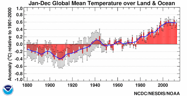
Figure \(\PageIndex{3}\) is a graph titled “Jan–Dec Global Mean Temperature over Land & Ocean.” The chart shows global temperature anomalies from approximately 1880 to 2010, measured relative to the 1901–2000 average.

The horizontal axis represents years, and the vertical axis shows temperature anomaly in degrees Celsius, ranging from about −1.0°C to +1.0°C. Red bars represent annual temperature anomalies, while a blue line shows the smoothed long-term trend. Gray error bars indicate uncertainty in the measurements.

From the late 1800s through the early 1900s, most temperature anomalies are negative, generally between −0.1°C and −0.5°C. Temperatures rise during the 1930s and 1940s, briefly reaching slightly positive values before leveling off and fluctuating around the average through the 1950s to 1970s.

Beginning in the late 1970s, a pronounced warming trend emerges. Temperature anomalies increase steadily through the 1980s, 1990s, and 2000s. By the end of the record, annual anomalies reach approximately +0.6°C to +0.7°C above the 1901–2000 average.

The graph highlights a clear long-term increase in global average temperatures, with the warmest years occurring in the most recent decades shown. A NOAA logo appears in the lower-left corner, and the source is identified as NCDC/NESDIS/NOAA.

Increasing levels of greenhouse gases results in rising global air temperatures. Global mean surface temperatures have increased roughly 1.53°F (0.85ºC) from 1880 to 2012. The annual trend in average global air temperature through December 2012 is depicted in Figure \(\PageIndex{3}\). The range of measurement uncertainty is indicated by the gray vertical bars. The temperature trends over the past 100-plus years in Figure \(\PageIndex{4}\) clearly indicate rising temperatures on all continents and over the oceans.

Figure \(\PageIndex{4}\): Global and Continental Temperature Change, 1900 - 2000. Data for the last hundred years already show clear trends in warming for the globe and continents. (CC BY-SA 4.0; Michael Ritter via The Physical Environment) 

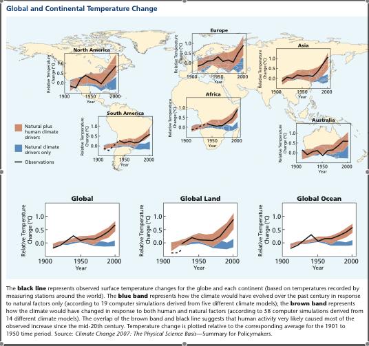
Figure \(\PageIndex{4}\) is an infographic titled “Global and Continental Temperature Change.” A world map serves as the background, with nine small graphs showing temperature trends for North America, South America, Europe, Africa, Asia, Australia, Global, Global Land, and Global Ocean from about 1900 to 2000. Each graph contains:

• A black line representing observed temperature changes.
• A brown shaded band representing climate model simulations that include both natural influences and human-caused factors.
• A blue shaded band representing simulations that include only natural climate drivers.

Across all regions, temperatures fluctuate during the early twentieth century and then rise substantially after about 1970. In most graphs, the observed temperatures closely follow the brown band, especially during the late twentieth century, while diverging from the blue band.

The largest increases appear in Asia, Europe, and Global Land, where temperatures rise by roughly 1°C or more by 2000. Global Ocean temperatures also increase but by a somewhat smaller amount. Africa, South America, Australia, and North America all show clear warming trends. A legend identifies:

• Brown: Natural plus human climate drivers
• Blue: Natural climate drivers only
• Black line: Observations

The caption explains that the observed temperature record aligns much more closely with model simulations that include human influences than with simulations based only on natural factors. The figure illustrates that most of the warming observed since the mid-twentieth century is consistent with the effects of human activities on climate.

The last decade, 2000-2009, ended on the second warmest year on record. The temperature anomaly map (Figure \(\PageIndex{5}\)) shows the departure from "normal" for the reference period of 1951 through 1980. Very little of the earth showed cooling while most experienced warming. The greatest warming occurred in the Arctic, coinciding with changes in surface albedo as annual sea ice diminishes.

Figure \(\PageIndex{5}\): 2000 - 2009 Temperature Anomaly. (CC BY-SA 4.0; Michael Ritter via The Physical Environment).

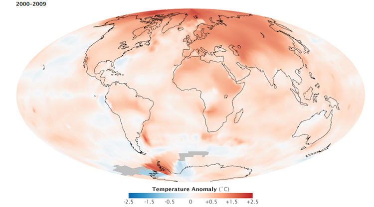
Figure \(\PageIndex{5}\) is a world map showing global temperature anomalies for 2000–2009 relative to a long-term average. The map displays areas that were warmer or cooler than average across Earth's land and ocean surfaces.

Most of the globe shows positive temperature anomalies, indicating warmer-than-average conditions. The strongest warming occurs at high northern latitudes, including northern North America, Greenland, northern Europe, and Siberia. These regions exhibit the largest temperature increases on the map.

Much of Africa, Europe, Asia, South America, and Australia also experienced above-average temperatures. Oceans generally show warming as well, though the magnitude is smaller than over many land areas.

A few localized regions, particularly in parts of the Southern Ocean near Antarctica and limited areas of the Pacific Ocean, display cooler-than-average temperatures.

A legend at the bottom indicates temperature anomalies ranging from approximately −2.5°C to +2.5°C. The map illustrates that warming during 2000–2009 was widespread globally, with the most pronounced increases occurring in the Arctic and other northern high-latitude regions.