3.1.8: Global Patterns of Insolation, Net radiation, and Heat

Insolation 

Patterns of insolation and net radiation which determine the location of plants, animals, climate, soils and other elements of our physical environment can be discerned from Figures \(\PageIndex{1}\) through \(\PageIndex{3}\). Figure \(\PageIndex{1}\) illustrates the latitudinal distribution of incoming solar radiation and outgoing terrestrial radiation. From approximately 35^o N to 35^o S latitude (the red area of the graph) there is a surplus of energy as incoming radiation exceeds outgoing. The blue regions indicate that there is more outgoing energy than incoming, yielding a net loss of energy from the Earth's surface. One might ask then why the middle to higher latitudes aren't getting colder through time as a result of the net loss, and the subtropical to equatorial regions getting constantly hotter due to the net gain. The reason is that the energy is redistributed by circulation of the atmosphere and oceans. Heat gained in the tropics is transported poleward by the global circulation of air and warm ocean currents to heat higher latitude regions. Cooler air from the higher latitudes and cold ocean currents push equatorward to cool the lower latitudes. This process of redistributing energy in the Earth system helps maintain a long-term energy balance.

Figure \(\PageIndex{1}\): Latitudinal Variation of the Radiation Balance (CC BY-SA 4.0; Michael Ritter via The Physical Environment) 

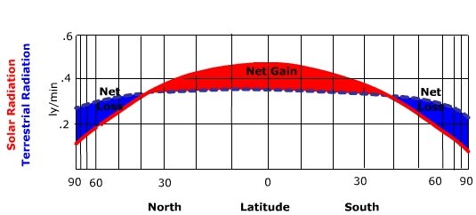
Figure \(\PageIndex{1}\) is a graph showing how solar radiation and terrestrial (Earth-emitted) radiation vary with latitude, and how their difference creates zones of energy gain and loss.

Axes and layout:

• The horizontal axis is labeled latitude, ranging from 90 degrees North on the left, through 0 degrees (the equator) in the center, to 90 degrees South on the right.
• The vertical axis represents the amount of radiation. Two types are shown: solar radiation (incoming) and terrestrial radiation (outgoing).

Lines and regions:

• One curve represents incoming solar radiation, which is highest near the equator and decreases toward both poles.
• Another curve represents outgoing terrestrial radiation, which varies less with latitude compared to solar radiation.
• The area between these two curves is shaded:
  • A central region near the equator is labeled “Net Gain.”
  • Regions toward both polar ends are labeled “Net Loss.”

Pattern and meaning:

• Near the equator, incoming solar radiation is greater than outgoing terrestrial radiation. This creates a surplus of energy (net gain).
• At higher latitudes (toward both the North and South poles), outgoing radiation exceeds incoming solar radiation. This creates a deficit of energy (net loss).
• There are transition points in mid-latitudes where the two curves intersect, representing locations where incoming and outgoing radiation are roughly balanced.

Figure \(\PageIndex{1}\) simplifies the geographic distribution of insolation. For the Earth as a whole, particular patterns can be accounted for by variation in surface features that impact insolation. Figure \(\PageIndex{2}\) illustrates that insolation maxima are found in the tropical and subtropical deserts of the earth. Here, high sun angles and a lack of cloud cover in desert regions allow much solar radiation to the surface. Insolation decreases to a minimum at the poles where low sun angles and the fact that the Sun doesn't rise above the horizon nearly half the year reduces annual insolation.

Figure \(\PageIndex{2}\): Annual global distribution of solar radiation (Kcal/cm²). (CC BY-SA 4.0; Michael Ritter via The Physical Environment).

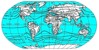
Figure \(\PageIndex{2}\) is a world map showing the global distribution of energy gain and loss using contour lines. The map includes all continents and oceans, with curved lines drawn across the surface representing equal values of energy surplus or deficit.

Numbers are placed along the contour lines, including values such as 200, 100, 70, 0, and −70. These values represent the balance between incoming solar radiation and outgoing terrestrial radiation at different locations on Earth.

Across the region near the equator, the contour values are highest, with numbers around 200. This indicates a strong net energy gain, meaning more solar energy is received than is lost. These high values extend across equatorial regions of South America, Africa, and Southeast Asia.

Moving toward mid‑latitudes, the contour values decrease. Around these regions, the values approach zero, indicating a balance between incoming and outgoing radiation.

Toward the higher latitudes near both the Northern and Southern Hemispheres, the contour values become smaller and then negative, such as −70. These areas indicate a net energy loss, where more energy is emitted to space than is received from the Sun.

The contour lines curve and shift slightly over land and ocean areas, showing regional variation in the magnitude of energy gain or loss.

Net radiation

Net radiation exhibits a different pattern from that of insolation. Figure \(\PageIndex{3}\) shows that maximum net radiation is found over the tropical and subtropical oceans. The sun angle is always high over the tropical oceans so the surface receives intense radiation throughout the year. With an high sun angle the albedo of the surface is low and absorption is high. However, the energy received is partitioned into warming the surface as well as evaporating water. The result is a lower surface temperature than one might expect with such high sun angles. Additionally, the high specific heat of water means that it takes much more energy to heat a unit mass of water than that of land, resulting in lower ocean surface temperatures. With lower surface temperatures the water surface does not radiate as much longwave radiation out to the atmosphere as nearby land at the same latitude. With much radiation coming in and little going out, the net value is large compared to land at the same latitude. Net radiation is at a minimum over the poles as the sunlight that comes in at a low angle is reflected from the ice-covered surface. Combined with the long polar night, very little net radiation is found at these latitudes.

Figure \(\PageIndex{3}\): Annual global distribution of net radiation (Kcal/cm²). (CC BY-SA 4.0; Michael Ritter via The Physical Environment).

Figure \(\PageIndex{3}\) is a world map showing curved lines that represent the global movement of energy across Earth. These lines indicate the transfer of heat from regions with energy surplus to regions with energy deficit.

Across the equatorial region, the lines begin where energy input is greatest. These areas correspond to low latitudes where incoming solar radiation exceeds outgoing radiation, creating a net energy gain.

From these low-latitude regions, the lines extend outward toward both the Northern and Southern Hemispheres. The lines curve as they move poleward, crossing over oceans and continents. This curvature reflects the pathways of atmospheric and ocean circulation systems that transport energy.

As the lines move toward mid‑latitudes and high latitudes, they reach regions where energy loss dominates. These higher latitude areas receive less incoming solar radiation and lose more energy to space.

The map shows multiple pathways of heat transfer, forming a continuous pattern connecting equatorial regions to polar regions. The density and direction of the lines indicate that energy is redistributed globally rather than remaining in one place.