1.7.1: Maps

What is a Map? 

A map is the fundamental tool of the geographer. With a map, one can illustrate the spatial distribution (i.e., geographic pattern) of almost any kind of phenomena. Maps provide a wide range of information. Currently with the application of GIS techniques to mapping, the depth of information that is presented has improved. The information collected to create a map is called spatial data. Any object or characteristic that has a location can be considered spatial data. Maps, by adding a spatial component to data not only attempt to answer the question what its characteristics are but also answer the question where something is. All spatial data has certain characteristics which are : location, attributes (descriptive information about a feature), spatial relationships, scale and resolution and representation (raster and vector data).  

1. Location - Specific geographic location that is expressed through coordinates like latitudes and longitudes.
2. Attributes - Descriptive information about a feature (name, area, population etc).
3. Spatial relationship - How the feature relates to each other in space (connectivity).
4. Scale and Resolution - The level of detail and the area covered by the data.
5. Representation - Vector data uses points lines and polygons to represent the data while raster data represents space as a grid of pixels (equal sized cells). 

Maps can primarily depict two kinds of data. Qualitative map data is in the form of a quality and expresses the presence or absence of the subject on a map, like the kind of vegetation present occupying a region. Quantitative map data is expressed as a numerical value, like elevation in meters, or temperature in degrees celsius. There are many different kinds of maps that serve quite different purposes.

Types of Maps

Reference Maps

Reference or navigational maps are created to help you navigate over the Earth surface. These kinds of maps show you where particular places are located and can be used to navigate your way to them. A street map or the common highway road map falls into this category.

Thematic Maps

Thematic maps are used to communicate geographic concepts like the distribution of densities, spatial relationships, magnitudes, movements etc. World climate or soils maps are notable examples of thematic maps. There are five common techniques for depicting geography data on a thematic map. The most common is a choropleth map that uses color to show variations in quantity, density, percent, etc. within a defined geographic area. Each color usually depicts a range of values.

Figure \(\PageIndex{1}\): Palmer Drought Index. (CC BY 4.0; Courtesy A. Dai & D. Shea via NCAR/UCAR Climate Data Guide).

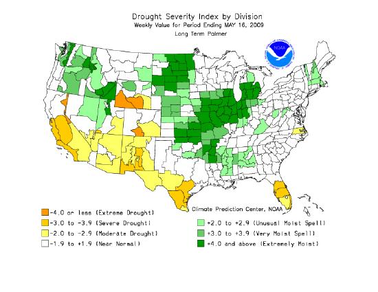
Figure \(\PageIndex{1}\) is a map of the United States labeled “Drought Severity Index by Division” for the week ending January 25, 2014. Different colors represent levels of dryness and moisture. Shades of orange indicate drought conditions, with darker orange showing more severe drought. Shades of green indicate wetter-than-normal conditions, with darker green showing extremely moist areas. Light or white areas represent near-normal conditions.

The map shows more intense drought conditions in parts of the western United States, especially in California and nearby regions. Some central areas show moderate drought, while parts of the eastern United States display wetter conditions. A legend at the bottom explains the color categories, ranging from extreme drought to extremely moist.

Defined areal units are colored on the Palmer Drought Index map in Figure\(\PageIndex{1}/) to show the pattern of dryness across the United States. Using administrative units presents a less realistic picture of the pattern of the distribution of natural phenomena. To overcome this, a variant of the choropleth map, the dasymetric map was created. This type of map employs special statistical methods and extra information to combine areas of similar values to depict geographic patterns on the map. The USDA's Plant Hardiness Zone Map is a dasymetric map.

Figure \(\PageIndex{2}\): USDA's Plant Hardness Zone map for North America (based on climate studies). (CC BY-SA 4.0; via U.S. Department of Agriculture).

Figure \(\PageIndex{2}\) is a map of North America labeled “USDA Plant Hardiness Zone Map.” It shows regions classified by average annual minimum temperature. Different colors represent temperature ranges, with a legend on the right listing zones from 1 to 11. Lower-numbered zones, shown in blues and purples, indicate colder regions with extremely low minimum temperatures, while higher-numbered zones, shown in yellows, oranges, and reds, indicate warmer regions.

The map shows colder zones concentrated in northern Canada and Alaska, while warmer zones appear in the southern United States and Mexico. Централь regions transition gradually between these extremes. This map helps identify which plants can survive winter temperatures in different locations.

An isarithmic map uses isolines, lines that connect equal values, to illustrate continuous data such as elevation, air pressure, and precipitation. Topographic maps shown in Figure \(\PageIndex{3}\) use contour lines to show elevation (height above sea level). Contour lines connect points of equal elevation above a specified reference, usually as sea level. The heavy brown contour lines with the elevation printed on them are called index contours. Intermediate contours are the lighter brown lines between index contours. Sometimes dashed lines called supplemental contours are used in areas of very low relief. Benchmarks are locations where the elevation has been surveyed. 

Figure \(\PageIndex{3}\): Sample Topographic map. (CC BY-SA 4.0; via USGS Monarch Lake).

Figure \(\PageIndex{3}\) shows a portion of a topographic map featuring very closely spaced contour lines around a labeled peak called Kiowa Peak. The contour lines form concentric patterns that indicate elevation. Near the center, contour labels such as 12,600 and 12,700 mark increasing elevation toward the peak.

The tightly packed contour lines indicate a steep slope in this area. Lighter shaded regions and small blue areas represent lower-lying features, likely water bodies. The map demonstrates how contour lines are used to represent changes in elevation and terrain shape.

Not only are natural features like mountains, valleys, streams and glaciers portrayed, but cultural features as well, like houses, schools, streets, and urbanized areas. 

Figure \(\PageIndex{4}\): Major earthquakes felt in Canada. (CC BY-SA 4.0; Courtesy Michael E. Ritter, The Physical Environment).

Figure \(\PageIndex{4}\) is a map of Canada showing earthquake activity and population distribution. The background uses color shading to represent population density, with lighter areas indicating low population and darker areas showing higher population, mainly along southern regions near the United States border.

Red circles of varying sizes are placed across the map to represent major earthquake locations. Larger circles indicate areas with higher earthquake activity or greater impact. These circles are concentrated along the western coast of Canada, especially in British Columbia, and appear in fewer locations across central and eastern Canada.

A legend at the bottom explains the population density scale using color shading and identifies the red circles as major earthquakes by area affected. The map highlights that earthquakes are more common along the western edge of Canada, where tectonic activity is higher.

Proportional or graduated circle maps are another way of depicting geographic information on a map. Figure \(\PageIndex{4}\) is a map that shows population density of Canada as colored polygons and the distribution of major earthquakes felt throughout the country. Graduated circles indicate the area over which the earthquakes were felt. This map was created using a geographic information system which has the capability of overlying different kinds of spatial data to show the relationships between them.

Dot maps use dots to illustrate the presence of the phenomenon on a map. A dot may equate to one or several units of measurement. Dot maps are especially useful in visualizing the frequency of occurrence or density of a mapped variable.

Figure \(\PageIndex{5}\): Dot map of agricultural chemical use. (CC BY-SA 4.0; Michael E. Ritter via USDA & The Physical Environment)

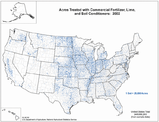
 Figure \(\PageIndex{5}\) is a map of the United States titled “Acres Treated with Commercial Fertilizer, Lime, and Soil Conditioners: 2002.” The map uses small blue dots to represent treated farmland, with a note indicating that one dot equals 25,000 acres.

The blue dots are distributed across the country, with the highest concentration in the Midwest and central Plains regions, indicating large areas of agricultural activity and soil treatment. Moderate concentrations appear in parts of the Southeast, while relatively few dots are visible in the western United States.

State boundaries and county divisions are outlined, and Alaska is shown in a small inset. A label at the bottom indicates a total of approximately 248 million acres treated, based on sample data. The map helps users compare regional patterns in land use and agricultural practices across the United States.

Isolines

Isarithmic maps use isolines to depict the geographic pattern of Earth phenomena. An isoline is a line that connects points of equal value. For instance, the brown contour lines on a topographic map connect points of equal elevation. Isobars are used to show the distribution of air pressure . Some common isolines encountered in physical geography are:

• isotherm - a line connecting points of equal temperature.
• isohyet - a line that connects points of equal precipitation.
• isophene - a line representing points where biological events occur at the same time, such as crops flowering.
• isopleth - a line connecting points of equal numerical value, like population.
• isotach - a line of equal wind speed.
• isobath - a line representing points of equal water depth.

Figure \(\PageIndex{6}\): Isobars on a weather map depicting pressure pattern over United States (CC BY-SA 4.0; Courtesy Pearson Scott Foresman)

Figure \(\PageIndex{6}\) is a weather map of the United States showing atmospheric pressure patterns using contour lines called isobars. These curved lines are labeled with values such as 985, 990, 995, 1000, 1015, and 1020, indicating air pressure in millibars.

A low-pressure system is visible in the western United States, with tightly packed, circular isobars centered near values around 985, indicating stronger weather activity. A high-pressure system appears in the southeastern United States, with isobars labeled around 1020, indicating more stable conditions.

Cities such as Los Angeles (LAX), Denver (DEN), Indianapolis (IND), and Miami (MIA) are marked for reference. The map demonstrates how pressure systems are distributed across the country and how isobars are used to identify areas of low and high pressure. 

A few "rules" apply to isolines. First, there is a set interval between consecutive isolines called the isoline interval. For example, the map in Figure \(\PageIndex{6}\) uses isobars to depict the distribution of air pressure. A four millibar interval was used to draw them. Second, two different isolines cannot cross each other. If they did, it would mean two different values are at the same location. Third, values inside a closed isoline are either higher or smaller than those outside.

Figure \(\PageIndex{7}\): The land surface and how its depicted on a topographic map. (CC BY-SA 4.0; USGS courtesy  Michael E. Ritter, The Physical Environment).

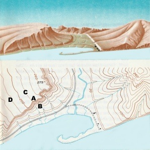
Figure \(\PageIndex{7}\) contains two related views of the same landscape: a 3D perspective at the top and a topographic map below. The upper portion shows a mountainous area with ridges, valleys, and a lake in the foreground. The terrain slopes upward from the water toward a peak, with curved ridges and a narrow valley cutting through the area.

The lower portion shows a contour map of the same region. Curved contour lines represent elevation, with lines closer together indicating steeper slopes. A stream flows through the valley and into the lake. Points labeled A, B, C, and D mark specific locations on different parts of the terrain, such as the valley floor, slopes, and higher elevations.

Together, the image demonstrates how three-dimensional landforms are represented using contour lines on a two-dimensional map, helping users connect real landscapes with map features.

Because the interval between isolines is constant, their spacing gives a visual indication of the change that occurs over a given distance, called a gradient. The more closely spaced the isolines, the larger is the gradient. For example, the spacing of contour lines between A to B on the topographic map shows a much steeper hill slope gradient than does the spacing of the contour lines between points C to D.

Map Scale

Map scale is the relationship between distance on a map and distance in the real world. There are several ways to specify map scale. Often we find the scale of a map expressed in words like, "one inch equals one mile". You’ve most likely seen map scale depicted with a graphic, like a bar divided up into segments. The length of a segment represents some distance on the Earth. We can specify scale as a representative fraction as well. These fractions often appear as follows:

1:24000

The fraction means that one unit of measurement on a map represents 24000 units in the real world. It’s important to remember that the same units of measurement are on either side of the colon. That is, 1 inch represents 24000 inches, or 1 centimeter represents 24000 centimeters. To calculate the distance between two points, one simply measures the map distance and multiplies it by the number of "real world" units. For example, if the measured distance between two points on a map with a scale of 1:62500 is 2.4 inches, then the real world distance is 2.4 times 62500 or 150000 inches. It’s hard to think how far that really is so convert it to miles. To do so simply take 150000 and divide by the number of inches in a mile which is 63360. So, the distance between the two points is about 2.37 miles.

Scale Categories

Map scales are grouped into small, medium and large categories. Large scale maps, such as 1:24000 scale maps show a smaller area in great detail. They are useful for showing the locations of buildings and other features important to engineers and planners. Medium scale maps, (1:62500) are good for agricultural planning where less detail is required. Small scale maps have the least detail but show large areas. These are useful for extensive projects at regional levels of analysis. You can easily see the impact of map scale on the information in figures \(\PageIndex{8a}\) through \(\PageIndex{8c}\) below.

Figure \(\PageIndex{8a}\): Scale 1:240001 inch = 2000feet Area Shown: 1 square mile. (CC BY-SA 4.0; U.S.G.S.Topographic Maps, 1969 via  Michael E. Ritter , The Physical Environment).

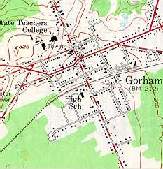
Figure \(\PageIndex{8a}\) is a detailed topographic map of a town labeled “Gorham.” The map shows streets, buildings, and nearby land features using symbols and contour shading. Dark lines and labels represent roads forming a grid-like street pattern across the town. Small black shapes and dots indicate buildings and developed areas. Green shaded regions surrounding the town represent vegetated or forested areas, while lighter areas show developed land. A feature labeled “High School” appears near the center-left of the town. A contour marking labeled “326” indicates elevation in feet, showing a small area of higher ground.This map demonstrates how topographic maps combine elevation, land cover, and human features such as roads and buildings to provide a detailed understanding of both natural terrain and settlement patterns. 

Figure \(\PageIndex{8b}\): Scale 1:625001 inch = nearly 1 mile Area Shown: 6 3/4 square miles. (CC BY-SA 4.0; via U.S.G.S Topographic Maps, 1969. Michael E. Ritter, The Physical Environment).

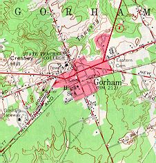
Figure \(\PageIndex{8b}\) is a detailed topographic map of the Gorham area. It shows roads, buildings, vegetation, and elevation using color shading and symbols. Red and black lines indicate major and minor roads forming a network through the town. Small black shapes represent buildings and developed areas. Green shaded regions indicate forested or vegetated land, while white or light-colored areas represent developed or open land. Contour lines, shown as thin brown curves, indicate changes in elevation, with closer lines representing steeper slopes. A stream or water feature is visible running through part of the map, connecting to nearby lower land areas. This map demonstrates how multiple layers—terrain, vegetation, water, and human features—are combined to help users understand both the physical landscape and how people use the land.

Figure \(\PageIndex{8c}\): Scale 1:250,000, 1 inch = nearly 4 miles, Area Shown: 107 square miles (CC BY-SA 4.0; U.S.G.S.Topographic Maps, 1969 Michael E. Ritter, The Physical Environment).

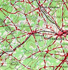
Figure \(\PageIndex{8c}\) is a detailed topographic map showing the Gorham and Westbrook areas along with surrounding regions. The map combines multiple layers of information, including roads, elevation, vegetation, and place names. Bold red lines represent major highways and transportation routes connecting towns such as Gorham, Westbrook, Buxton, and nearby areas. Thin black lines show smaller roads and local streets. Numerous place names are labeled across the map, including Gorham at the center and surrounding communities. Green shading indicates forested or vegetated land, while lighter areas represent developed or open land. Brown contour lines curve across the map and are labeled with elevation values such as 250 and 300, indicating height in feet. The spacing of the contour lines varies, with closer lines showing steeper terrain and wider spacing indicating gentler slopes. Blue lines and shapes represent streams, rivers, or small water bodies flowing through valleys and lower elevations. The map demonstrates how transportation networks, elevation, and land cover interact across a larger geographic region.

Concept Check \(\PageIndex{1}\)

Notice in Figure \(\PageIndex{8a}\)(above) that black squares have been used to depict individual buildings in the downtown of Gorham. Why hasn't this been done in Figure \(\PageIndex{8c}\)?

Answer

At the reduced scale of 1:62500, it is impossible to show the same level of detail as that of a map of a larger scale (1:24000). Small features like individual buildings in the downtown are too small at this scale to show each of them. If a cartographer tried, the downtown area would be covered in black. Instead, a pinkish color is used to depict urban area.

Map Projections

A map projection is a method of portraying the curved surface of the Earth on a flat planar surface of a map. Projections are created to preserve one or several measurements of the following qualities:

• Area
• Shape
• Direction
• Bearing
• Distance
• Scale

Each projection handles the conversion of these metric properties from the curved surface of a globe to the flat surface of map differently.

Figure \(\PageIndex{9}\): Visualizing a map projection ( CC BY-SA 4.0; Courtesy Michael E. Ritter, The Physical Environment)

The purpose of the map is of primary importance in choosing a projection to illustrate spatial patterns of Earth phenomena. Tangent and secant are terms used in map projection to describe how a geometric surface (like a cone, cylinder, or plane) interacts with the globe. This contact determines where on the resulting flat map there is zero distortion. Figure \(\PageIndex{10}\) illustrates the concept of tangents and secants. 

• Tangent: A tangent map projection occurs when the projection surface touches the globe at a single point or along a single line. The area of contact is known as the standard line in the case of cylinders or cones or point of tangency for planes. At this point or line, the scale is true and there is no distortion. Distortion increases as we move away from the point or line of tangency. 

• Secant: A secant map projection occurs when the projection surface intersects or slices through the globe. This creates two standard lines where the surface meets the globe. On a secant projection, the scale is true and distortion is minimized along both of these lines. This method is commonly used to average out and reduce distortion over a wider area between the two standard lines, making it more useful for mapping large regions than a tangent projection.

Figure \(\PageIndex{10}\): Comparison of Cartographic Surface Development.  (CC BY-SA 4.0; US government, Clindberg, Palosirkka, via Wikimedia Commons).

Figure \(\PageIndex{10}\) compares three types of map projections—cylindrical, conic, and azimuthal—and shows how each represents Earth’s curved surface on a flat map. Each projection type is illustrated using a globe and a geometric surface (a cylinder, cone, or flat plane) wrapped around it.

In the cylindrical projection (labeled φ = 0 degrees), the globe is wrapped by a cylinder. The red line marks the standard parallel where distortion is minimized. Areas farther from this line show increasing scale expansion, meaning features appear stretched.

In the conic projection (labeled 0 degrees < φ < 90 degrees), the globe is wrapped by a cone. A curved red line marks the standard parallel. Distortion is lowest along this line and increases as distance from it grows. The resulting map appears fan-shaped.

In the azimuthal projection (labeled φ = 90 degrees), a flat plane touches the globe at a single point, usually at the pole. That point has the least distortion, while areas farther away experience increasing distortion.

The diagram also compares two projection methods:

• Tangent projections, where the surface touches the globe at one line or point, resulting in scale expansion away from that contact.
• Secant projections, where the surface cuts through the globe, creating two lines of reduced distortion and areas of scale compression between them.

The diagram demonstrates how different projection methods affect accuracy in terms of distance, shape, and scale across a map.

For instance, the Mercator projection illustrated in Figure \(\PageIndex{10}\) was long used for navigation or maps of equatorial regions. The cylindrical Mercator projection mathematically projects the globe onto a cylinder tangent to the Equator. Large areas become distorted which increases toward away from the Equator. Distances are true only along the Equator, special scales are provided for other latitudes for measurement.

Figure \(\PageIndex{11}\): Cylindrical Mercator projection. (Public Domain; Courtesy USGS).

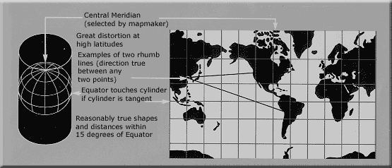
Figure \(\PageIndex{11}\) shows a world map using a cylindrical map projection centered on a selected central meridian. The map includes a grid of latitude and longitude lines forming a rectangular pattern across the globe.

Text on the image explains key characteristics of this projection. It notes that distortion increases at high latitudes, meaning regions near the poles appear stretched compared to areas near the equator. The map also shows examples of rhumb lines, or constant compass direction paths, drawn as straight or slightly curved lines connecting two points.

Additional text states that the equator is where the cylinder touches the globe in a tangent projection. As a result, shapes and distances are shown more accurately within about 15 degrees of the equator, while distortion increases farther away.

A small globe diagram on the left illustrates how a cylinder wraps around Earth to create the projection, helping explain how the flat map is formed.

The Robinson projection shown in Figure \(\PageIndex{11}\) uses tabular coordinates rather than mathematical formulas to make Earth features look the "right" size and shape. A better balance of size and shape result is a more accurate picture of high-latitude lands like Russia, Soviet and Canada. Greenland is truer to size but compressed.

Figure \(\PageIndex{12}\): Robinson projection. (Public Domain; via USGS).

Figure \(\PageIndex{12}\) shows a world map using a cylindrical map projection centered on a selected central meridian chosen by the mapmaker. The map includes a grid of latitude and longitude lines forming a rectangular layout.

A smaller diagram on the left shows a globe with labeled latitudes from 0° at the equator to 90° at the poles. Text explains that the central meridian is slightly shorter than the equator, measuring about 0.53 times its length, and that the equator appears as the longest horizontal line on the map.

The map on the right shows continents stretched horizontally, with meridians (north–south lines) curving inward, forming a concave shape, while remaining evenly spaced. This illustrates how the projection alters the shape and distances of locations.

The diagram demonstrates how cylindrical projections represent Earth by flattening a curved surface, and highlights how distortion affects the spacing and shape of latitude and longitude lines.

Optional Reading \(\PageIndex{1}\)

• For a complete reference of the symbols commonly used in topographic maps, visit the USGS Topographic Map Symbols guide, which provides detailed explanations of map markings and their meanings.
• For a better understanding of how maps represent the curved surface of Earth on a flat surface, explore the Map Projections from the United States Geological Survey. This guide explains different types of map projections and how each one affects the way distance, area, and shape are shown on a map.